
Probability And Statistics For Deep Learning
Interview-Ready Notes
Organization: DataLogos
Date: 04 Mar, 2026
Probability & Statistics for Deep Learning – Study Notes
Target audience: Beginners | Goal:
End-to-end learning and interview-ready
Difficulty: Beginner-friendly (assumes basic
algebra)
Estimated time: ~45 min read / ~1.5 hours with
exercises
Pre-Notes: Learning Objectives & Prerequisites
Learning Objectives
By the end of this note you will be able to:
- Define random variables, expectation, variance, and common distributions (Bernoulli, Gaussian) and explain their role in deep learning.
- Apply Bayes’ theorem and maximum likelihood estimation (MLE) to simple ML/DL scenarios.
- Explain the bias–variance tradeoff and how it connects to overfitting and underfitting.
- Use basic information-theory concepts (entropy, KL divergence) in the context of loss functions and model comparison.
- Answer common interview questions on probability and statistics with correct, concise answers and avoid standard traps.
Prerequisites
| You should know… | If you don’t… |
|---|---|
| Basic algebra (sums, products, exponents) | Review high-school algebra |
| What a function and derivative are | See Calculus for Deep Learning notes |
| High-level idea of “learning from data” | Skim Deep Learning from Scratch intro |
Where this fits: This topic is part of Phase 1: Mathematical Foundations. It builds on basic algebra and feeds into Loss Functions, Regularization, Optimization, and Information-Theory-based losses (e.g., cross-entropy, KL divergence) in later phases.
1. What is Probability & Statistics in the Context of Deep Learning?
Probability is the mathematics of uncertainty: it lets us quantify how likely outcomes are when we don’t know the result in advance. Statistics is the practice of learning from data: estimating unknown quantities, testing hypotheses, and making decisions under uncertainty.
In deep learning, we constantly deal with uncertainty: noisy data, random initialization, stochastic gradients, and predictions we want to interpret as probabilities (e.g., “80% chance this is a cat”). Probability gives us the language and tools to model and optimize under this uncertainty.
Simple Intuition
Think of training a model to predict whether an image is a cat or a dog:
- We don’t have a fixed rule “pixel pattern X ⇒ cat”; we have randomness (lighting, angle, breed).
- We treat the label as random (given the image) and the data as a random sample.
- We use probability to define “how wrong” a prediction is (loss) and statistics to estimate parameters (e.g., weights) from data.
Formal Definition (Interview-Ready)
Probability provides the formalism for random variables, distributions, and expectations used in loss functions, regularization, and sampling. Statistics provides estimation (e.g., MLE), the bias–variance tradeoff, and evaluation under uncertainty—all central to designing and training deep learning models.
2. Why Do We Need Probability & Statistics for Deep Learning?
Traditional rule-based systems assume deterministic inputs and outputs. ML/DL instead assumes data and labels are (or can be modeled as) random. Probability and statistics are needed to:
- Define loss functions (e.g., cross-entropy from likelihood, MSE from Gaussian assumption).
- Justify and derive algorithms (e.g., gradient descent as MLE under a Gaussian noise model).
- Reason about generalization (bias–variance, overfitting).
- Compare and calibrate models (entropy, KL divergence, confidence).
Key Reasons
| Reason | Role in DL |
|---|---|
| Uncertainty | Predictions as probabilities; dropout and sampling as random processes |
| Loss design | Cross-entropy, MSE, and many losses come from probabilistic assumptions |
| Estimation | MLE/MAP frame for learning weights from data |
| Evaluation | Variance of metrics, confidence intervals, A/B tests |
| Theory | Bias–variance, PAC-style bounds, information-theory arguments |
Real-World Problems Where This Shows Up
| Domain | How probability/statistics appears |
|---|---|
| Classification | Output as class probabilities; cross-entropy loss |
| Regression | MSE as MLE under Gaussian noise; uncertainty estimates |
| Generative models | VAEs, GANs, diffusion—all use distributions and sampling |
| Reinforcement learning | Policies as distributions; exploration vs exploitation |
| NLP | Language models as probability distributions over sequences |
3. Core Building Block: Random Variables, Distributions, Expectation & Variance
The core building blocks are random variables, probability distributions, and their summaries: expectation and variance. These underpin loss functions, initialization, and evaluation in DL.
Random Variables
- Discrete random variable \( X \): takes values in a countable set (e.g., class labels 1,…,K). Described by a probability mass function (PMF) \( P(X = x) \).
- Continuous random variable \( X \): takes values in an interval or the real line. Described by a probability density function (PDF) \( p(x) \) with \( \int p(x)\,dx = 1 \).
Interview-ready: A random variable is a variable whose value is determined by chance; in DL we often treat data, labels, and sometimes weights as random variables.
Common Distributions in DL
| Distribution | Type | Use in DL |
|---|---|---|
| Bernoulli | Discrete | Single binary outcome (e.g., one class probability) |
| Categorical | Discrete | Multi-class labels; softmax outputs |
| Gaussian (Normal) | Continuous | Regression noise; initialization; variational inference |
| Uniform | Continuous | Random initialization; sampling |
Bernoulli: \( P(X=1) = p,\; P(X=0) = 1-p \). Used for binary classification (one probability per example).
Gaussian: \( p(x) = \frac{1}{\sqrt{2\pi\sigma^2}} \exp\bigl(-\frac{(x-\mu)^2}{2\sigma^2}\bigr) \). Mean \( \mu \), variance \( \sigma^2 \). Used for regression (MSE = MLE under Gaussian noise), and often for weight priors/initialization.
Expectation and Variance
- Expectation (mean): \( \mathbb{E}[X] \) —
“average value” of \( X \) in the long run.
- Discrete: \( \mathbb{E}[X] = \sum_x x\, P(X=x) \).
- Continuous: \( \mathbb{E}[X] = \int x\, p(x)\,dx \).
- Discrete: \( \mathbb{E}[X] = \sum_x x\, P(X=x) \).
- Variance: \( \mathrm{Var}(X) = \mathbb{E}[(X - \mathbb{E}[X])^2] = \mathbb{E}[X^2] - (\mathbb{E}[X])^2 \) — spread around the mean.
- Standard deviation: \( \sigma = \sqrt{\mathrm{Var}(X)} \).
In DL, expectation appears in loss (e.g., expected loss over data), and variance appears in bias–variance tradeoff, gradient variance (SGD), and evaluation (e.g., variance of accuracy).
Covariance and Correlation
- Covariance: \( \mathrm{Cov}(X,Y) = \mathbb{E}[(X - \mathbb{E}[X])(Y - \mathbb{E}[Y])] \). Measures linear association.
- Correlation: \( \rho_{X,Y} = \frac{\mathrm{Cov}(X,Y)}{\sigma_X \sigma_Y} \in [-1, 1] \). Scale-invariant measure of linear relationship.
Used in DL for understanding feature relationships, whitening, PCA, and some regularization ideas.
In a Nutshell
Core idea: Random variables and their distributions (especially Bernoulli and Gaussian) plus expectation and variance form the language in which we define losses, priors, and generalization. Covariance/correlation extend this to multiple variables (e.g., features).
Think About It
Before moving on: Why might we model regression targets as Gaussian? What would the “most likely” prediction be under that model?
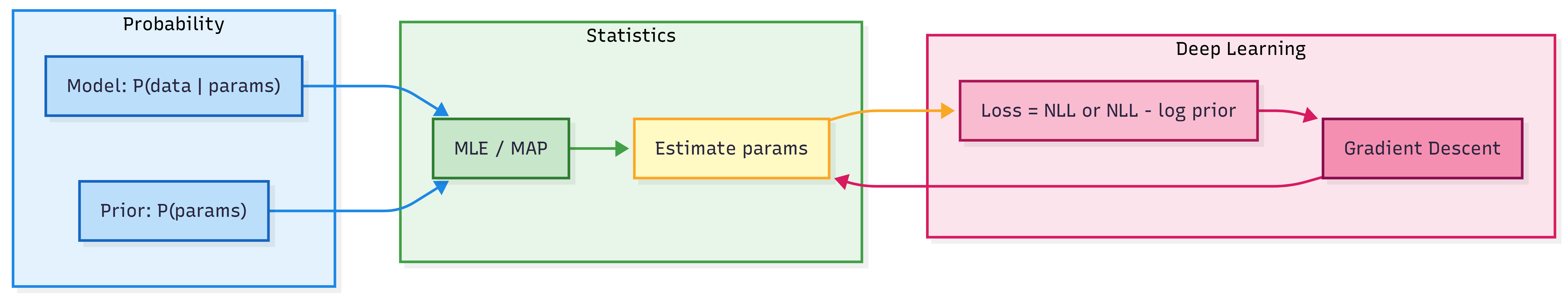
4. Process: From Probability to Learning (Bayes, MLE, Loss)
A compact “process” view of how probability and statistics connect to learning:
- Model the data (and optionally parameters) with probability distributions.
- Define likelihood (probability of data given parameters) or posterior (Bayes).
- Estimate parameters by maximizing likelihood (MLE) or posterior (MAP).
- Implement the negative log-likelihood as the loss and minimize it (e.g., gradient descent).
Bayes’ Theorem
\[ P(A \mid B) = \frac{P(B \mid A)\, P(A)}{P(B)} \]
- Prior \( P(A) \): belief before seeing data.
- Likelihood \( P(B \mid A) \): probability of data given the hypothesis/parameter.
- Posterior \( P(A \mid B) \): updated belief after seeing data.
In DL: MAP (maximum a posteriori) = maximize \( P(\text{params} \mid \text{data}) \propto P(\text{data} \mid \text{params})\, P(\text{params}) \). A Gaussian prior on weights gives L2 regularization.
Maximum Likelihood Estimation (MLE)
- Likelihood \( L(\theta) = P(\text{data} \mid \theta) \).
- MLE: \( \hat{\theta} = \arg\max_\theta L(\theta) \).
- In practice we often minimize negative log-likelihood (NLL) because log turns products into sums and many losses are NLL under a distributional assumption.
| Assumption | NLL loss | Typical use |
|---|---|---|
| Bernoulli per output | Binary cross-entropy | Binary classification |
| Categorical | Cross-entropy | Multi-class classification |
| Gaussian noise | MSE (up to constants) | Regression |
Interview tip: Cross-entropy loss is the negative log-likelihood of the correct class under the model’s predicted distribution. MSE is MLE for regression under i.i.d. Gaussian noise.
In a Nutshell (Process)
From probability to learning: Choose a distribution for the data (e.g., categorical for classification, Gaussian for regression), write the likelihood, then minimize NLL—that’s your loss. Bayes adds a prior; MAP gives regularization (e.g., L2).
5. Key Sub-Topics (Deep Dive)
| # | Sub-topic | What it is | DL relevance |
|---|---|---|---|
| 1 | Random variables & distributions | Formal description of uncertain quantities | Labels, outputs, and sometimes weights as random |
| 2 | Expectation & variance | Mean and spread of a distribution | Loss = expected loss; variance in bias–variance and SGD |
| 3 | Covariance & correlation | Linear dependence between variables | Features, PCA, data preprocessing |
| 4 | Bayes’ theorem | Update belief from data | MAP = MLE + prior; L2 from Gaussian prior |
| 5 | MLE | Estimate parameters by maximizing likelihood | Most supervised learning as minimizing NLL |
| 6 | Bias–variance tradeoff | Decomposition of generalization error | Overfitting vs underfitting; model complexity |
| 7 | Entropy & KL divergence | Information-theory measures | Cross-entropy, label smoothing, variational inference |
6. Comparison: Probability vs Statistics (and How They Work Together)
| Aspect | Probability | Statistics |
|---|---|---|
| Focus | Mathematical model of randomness | Inference from data |
| Typical question | “If the model is X, what outcomes do we expect?” | “Given data, what can we say about the model?” |
| In DL | Defining distributions, losses, sampling | Estimating weights, evaluating metrics, confidence |
They work together: probability specifies the model (e.g., “labels are categorical given logits”); statistics uses data to choose parameters (e.g., MLE/MAP) and assess performance.
7. Common Types / Variants
- Discrete vs continuous distributions — Discrete for classification (Bernoulli, categorical); continuous for regression and latent variables (Gaussian, uniform).
- Frequentist vs Bayesian — MLE (point estimate) vs posterior/MAP (prior + likelihood); in DL we often use point estimates with implicit or explicit regularization (e.g., dropout, weight decay).
- Parametric vs non-parametric — Parametric: fixed family (e.g., Gaussian); non-parametric: flexible (e.g., histograms). Most DL models are parametric with many parameters.
- Univariate vs multivariate — One variable vs many; multivariate Gaussians and covariance matrices appear in whitening, VAEs, and some initializations.
8. Bias–Variance Tradeoff (Critical for DL)
Generalization error can be decomposed (conceptually) into:
Bias: Error from wrong assumptions (underfitting).
Variance: Error from sensitivity to the training sample (overfitting).
Irreducible error: Noise in the data.
High bias → underfitting (e.g., too simple model).
High variance → overfitting (e.g., memorizing training set).
In deep learning we try to reduce variance (regularization, dropout, more data) while keeping bias manageable (capacity, architecture). We rarely compute bias/variance explicitly; the tradeoff guides design choices.
In a Nutshell
Bias–variance: Simple models tend to underfit (high bias); complex models tend to overfit (high variance). Good ML/DL balances the two through model choice, regularization, and data.
Self-Check
Q: If your model has high training error and high
test error, is the main issue bias or variance?
A: High bias (underfitting). High
variance would typically show as low training error but high test
error.
9. Information Theory Basics (Entropy, KL Divergence)
- Entropy \( H(P) = -\sum_x P(x)\log P(x) \) (discrete). Measures “uncertainty” or “surprise” of a distribution. Higher entropy = more uncertainty.
- Cross-entropy \( H(P, Q) = -\sum_x P(x)\log Q(x) \). Average bits when we use \( Q \) to encode \( P \). In classification, cross-entropy loss uses true label distribution \( P \) and predicted \( Q \).
- KL divergence \( D_{\mathrm{KL}}(P \| Q) = \sum_x P(x)\log\frac{P(x)}{Q(x)} \). Asymmetric measure of “distance” from \( Q \) to \( P \). \( D_{\mathrm{KL}}(P \| Q) = H(P,Q) - H(P) \).
In DL: Cross-entropy is the standard classification loss. KL divergence appears in VAEs (regularizer), distillation, and label smoothing.
Interview tip: Minimizing cross-entropy with respect to model \( Q \) is equivalent to minimizing KL divergence from true \( P \) to \( Q \), because \( H(P) \) does not depend on the model.
10. FAQs & Common Student Struggles
Q1. What is the difference between probability and statistics?
Probability studies random phenomena and their mathematical models (distributions, expectations). Statistics uses data to estimate parameters, test hypotheses, and make decisions. In DL we use probability to define models and losses, and statistics to fit and evaluate them.
Q2. Why is the normal (Gaussian) distribution so common in DL?
It is mathematically convenient (closed-form MLE, central limit theorem), and assuming Gaussian noise on regression targets leads directly to MSE loss. Many initializations and variational methods also use Gaussians.
Q3. What is MLE in one sentence?
MLE chooses the parameter values that make the observed data most probable (maximize likelihood or equivalently minimize negative log-likelihood).
Q4. How does Bayes’ theorem connect to regularization?
MAP maximizes posterior = likelihood × prior. A Gaussian prior on weights yields an L2 penalty in the loss; a Laplace prior yields L1. So “regularization” can be seen as encoding a prior.
Q5. What is the bias–variance tradeoff in practice?
Bias = underfitting (model too simple). Variance = overfitting (model too sensitive to training set). We balance them by model capacity, regularization, and data size.
Q6. Why cross-entropy for classification and MSE for regression?
Cross-entropy is the NLL for a categorical (or Bernoulli) model of labels—the right probabilistic assumption for classification. MSE is the NLL for regression under i.i.d. Gaussian noise—the standard assumption for regression.
Q7. What is KL divergence used for in DL?
VAEs use KL as a regularizer (latent prior vs posterior). Distillation uses KL between teacher and student outputs. Label smoothing can be interpreted with KL/cross-entropy.
Q8. Is variance the same as variance in “bias–variance”?
Not exactly. Variance of a random variable is \( \mathrm{Var}(X) \). Variance in bias–variance is the variance of the estimator (e.g., predicted label) across different training sets. Both measure “spread,” but in different contexts.
Q9. What does “i.i.d.” mean and why does it matter?
I.i.d. = independent and identically distributed. We often assume training examples are i.i.d. samples. This justifies averaging loss over the dataset and many theoretical guarantees.
Q10. How do we “add” probability to a neural network?
We don’t add probability as an extra module—we interpret outputs as parameters of a distribution (e.g., logits → softmax → class probabilities; one output → mean of Gaussian for regression). Loss is then derived from that distribution (e.g., NLL).
11. Applications (With How They Are Achieved)
1. Classification (e.g., image, text)
Applications: Image classification, sentiment analysis, intent detection.
How probability/statistics achieve this:
- Model class label as categorical given input.
- Softmax outputs class probabilities; cross-entropy = NLL for that model.
- MLE (minimize cross-entropy) trains the network.
Example: ResNet for ImageNet: output = 1000-class distribution; loss = cross-entropy.
2. Regression (e.g., price, temperature)
Applications: Demand forecasting, sensor prediction, denoising.
How probability/statistics achieve this:
- Model target as Gaussian (or other continuous distribution) given input.
- MSE = NLL under i.i.d. Gaussian noise.
- MLE (minimize MSE) trains the network.
Example: Predicting house price: single output as mean; MSE loss.
3. Generative Models (VAE, diffusion)
Applications: Image generation, data augmentation, anomaly detection.
How probability/statistics achieve this:
- Define latent variables and prior (e.g., standard Gaussian).
- VAE: maximize ELBO = reconstruction (e.g., Bernoulli/Gaussian) + KL(prior || posterior).
- Diffusion: learn score / noise; sampling as reverse process.
Example: VAE: encoder → latent distribution; decoder → likelihood; loss = reconstruction + KL.
4. Uncertainty Estimation
Applications: Calibration, active learning, safety-critical systems.
How probability/statistics achieve this:
- Outputs as probabilities; use variance or entropy as uncertainty.
- Bayesian or ensemble methods for parameter/model uncertainty.
Example: Monte Carlo dropout: multiple forward passes; variance of predictions as uncertainty.
5. Regularization (L1/L2, dropout)
Applications: Better generalization, less overfitting.
How probability/statistics achieve this:
- L2 = Gaussian prior (MAP); L1 = Laplace prior.
- Dropout can be interpreted as Bayesian approximation or as noise.
Example: Weight decay in AdamW: equivalent to L2 prior in MAP view.
12. Advantages and Limitations (With Examples)
Advantages
1. Unified framework for loss and learning
Losses come from probabilistic assumptions (NLL), so we know what we are
optimizing.
Example: Cross-entropy is not arbitrary; it’s the right
loss for categorical labels under MLE.
2. Clear interpretation of outputs
Outputs as probabilities or distribution parameters support
decision-making and calibration.
Example: “80% cat” is interpretable; thresholding at
0.5 gives a decision rule.
3. Theory for generalization
Bias–variance and related ideas guide model and regularization
choices.
Example: Adding dropout when the model overfits is a
variance-reduction strategy.
4. Information theory for comparison
Entropy and KL give principled ways to compare distributions (e.g.,
teacher vs student).
Example: Knowledge distillation minimizes KL between
teacher and student outputs.
Limitations
1. Assumptions may be wrong
Gaussian noise or categorical labels may not hold.
Example: Heavy-tailed errors in finance can make MSE
suboptimal.
2. Full Bayesian inference is costly
Exact posterior is intractable in big networks; we use point estimates
or approximations.
Example: We use MLE/MAP and single forward pass, not
full posterior sampling.
3. Bias–variance is conceptual
We rarely compute bias and variance explicitly; we use them as
intuition.
Example: We observe overfitting and add regularization
without estimating variance numerically.
4. i.i.d. often violated
Time series, recommender systems, and non-stationary data break
i.i.d.
Example: Training on past sales and deploying on future
sales may have distribution shift.
13. Interview-Oriented Key Takeaways
- Probability = language of uncertainty (random variables, distributions, expectation, variance). Statistics = learning from data (MLE, MAP, bias–variance).
- Cross-entropy = NLL for classification (categorical/Bernoulli). MSE = NLL for regression under Gaussian noise.
- Bayes’ theorem links prior, likelihood, and posterior; MAP = likelihood + prior; Gaussian prior ⇒ L2.
- Bias–variance: Underfitting (bias) vs overfitting (variance); balance via capacity, regularization, data.
- Entropy = uncertainty; KL divergence = “distance” between distributions; both appear in loss and regularization (VAE, distillation).
- For interviews: define distributions, state MLE/MAP in one line, and connect loss (cross-entropy, MSE) to probability.
14. Common Interview Traps
Trap 1: “Is probability necessary for deep learning?”
Wrong: No, we just minimize loss.
Correct: Probability provides the justification for
loss functions (e.g., cross-entropy, MSE), regularization (priors), and
sampling. It’s the right language for uncertainty and
generalization.
Trap 2: “What loss do we use for classification?”
Wrong: We use accuracy or MSE.
Correct: We use cross-entropy (or
binary cross-entropy for binary). MSE is for regression. Accuracy is a
metric, not a differentiable loss.
Trap 3: “What is MLE?”
Wrong: Minimizing loss.
Correct: Maximum Likelihood Estimation
= choose parameters that maximize the probability of the observed data.
Minimizing NLL is equivalent to MLE.
Trap 4: “More parameters always mean more variance (overfitting).”
Wrong: Yes, always.
Correct: Generally more capacity can increase variance,
but with strong regularization or more data, large models can still
generalize. It’s a tradeoff, not a fixed rule.
Trap 5: “What is the difference between variance and bias?”
Wrong: Variance is spread of data; bias is
prejudice.
Correct: In bias–variance decomposition:
bias = error due to model class (underfitting);
variance = error due to sensitivity to the training
sample (overfitting).
Trap 6: “KL divergence is symmetric.”
Wrong: Yes, like distance.
Correct: No. \( D_{\mathrm{KL}}(P \| Q) \neq D_{\mathrm{KL}}(Q \| P) \) in general. It’s an asymmetric measure.
Trap 7: “We need a Bayesian network to use Bayes.”
Wrong: Yes.
Correct: Bayes’ theorem is a general rule for updating
belief. We use it in MAP (prior + likelihood), and in Bayesian neural
networks; we don’t need a special “Bayesian network” architecture to use
the theorem.
Trap 8: “Entropy is the same as cross-entropy.”
Wrong: Yes, both measure uncertainty.
Correct: Entropy \( H(P) \) is one distribution.
Cross-entropy \( H(P,Q) \) is two
(e.g., true vs predicted). Cross-entropy ≥ entropy; equality when \( P = Q \).
15. Simple Real-Life Analogy
Probability is like knowing the rules of the game (e.g., how a fair die behaves). Statistics is like watching many throws and then guessing whether the die is fair and what the chances are. In deep learning, we assume a “game” (e.g., labels drawn from a categorical distribution), and we use data (statistics) to learn the parameters of that game (weights).
Probability & Statistics in System Design – Interview Traps (If Applicable)
Trap 1: Assuming Training and Production Distributions Match
Wrong thinking: “Our training data is representative forever.”
Correct thinking:
- Data drift changes \( P(\text{input}) \) or \( P(\text{label} \mid \text{input}) \).
- Monitor input/output distributions and retrain or adapt when they shift.
Example: A classifier trained on daytime images may see different lighting in production; accuracy can drop.
Trap 2: Treating Point Estimates as True Probabilities
Wrong thinking: “The softmax output is the real probability.”
Correct thinking:
- Softmax outputs are model beliefs, often overconfident.
- Use calibration (e.g., temperature scaling, Platt scaling) if you need reliable probabilities for decisions.
Example: A model outputting 0.99 for “cat” may be overconfident; calibration can align it with empirical frequencies.
Trap 3: Ignoring Variance in Metrics
Wrong thinking: “We ran once and got 90% accuracy.”
Correct thinking:
- Metrics have variance (different splits, seeds).
- Report mean and standard deviation or confidence intervals, especially for small datasets.
Example: Reporting “90% ± 2%” is more honest than “90%” when variance is high.
Likely Interview Questions (Quick List)
- What is the difference between probability and statistics?
- Why cross-entropy for classification and MSE for regression?
- Explain MLE in one sentence.
- How does Bayes’ theorem connect to L2 regularization?
- What is the bias–variance tradeoff? Give an example of high bias and high variance.
- What is KL divergence? Where is it used in DL?
- Is KL divergence symmetric?
- What is the role of the Gaussian distribution in deep learning?
Elevator Pitch
30 seconds:
Probability gives us random variables, distributions, and
expectations—the language for uncertainty. Statistics gives us MLE and
bias–variance—how we learn and generalize. In DL, we use them to define
losses (e.g., cross-entropy, MSE), justify regularization (priors), and
reason about overfitting and underfitting.
2 minutes:
We model data and labels with probability distributions. For
classification we use categorical/Bernoulli and minimize negative
log-likelihood, which is cross-entropy. For regression we often assume
Gaussian noise, so MLE gives MSE. Bayes’ theorem links prior and
likelihood to the posterior; MAP with a Gaussian prior gives L2
regularization. The bias–variance tradeoff explains underfitting vs
overfitting: we balance model complexity and regularization. Information
theory gives entropy and KL divergence, used in VAEs and distillation.
So probability tells us what we optimize; statistics tells us how we
learn from data and evaluate.
Interview Gold Line
“Probability tells us what we’re optimizing (e.g., NLL); statistics tells us how we learn and evaluate from data. In deep learning, both are essential—not optional.”
Diagram: From Data to Loss (Conceptual Flow)
One-Page Cheat Sheet
| Concept | Definition / formula |
|---|---|
| Random variable | Variable whose value is determined by chance (discrete: PMF; continuous: PDF). |
| Expectation \( \mathbb{E}[X] \) | Mean; \( \sum x\, P(X=x) \) or \( \int x\, p(x)\,dx \). |
| Variance \( \mathrm{Var}(X) \) | \( \mathbb{E}[(X - \mathbb{E}[X])^2] \); spread. |
| Bernoulli | \( P(X=1)=p \); binary outcome. |
| Gaussian | \( p(x) \propto \exp(-(x-\mu)^2/(2\sigma^2)) \); mean \( \mu \), variance \( \sigma^2 \). |
| Bayes | \( P(A\mid B) = P(B\mid A)P(A)/P(B) \). |
| MLE | \( \hat{\theta} = \arg\max_\theta P(\text{data}\mid\theta) \); same as minimize NLL. |
| MAP | Maximize \( P(\text{params}\mid\text{data}) \propto \text{likelihood} \times \text{prior} \); Gaussian prior ⇒ L2. |
| Bias–variance | Error = bias (underfitting) + variance (overfitting) + noise. |
| Entropy \( H(P) \) | \( -\sum P\log P \); uncertainty. |
| Cross-entropy \( H(P,Q) \) | \( -\sum P\log Q \); classification loss. |
| KL divergence | \( D_{\mathrm{KL}}(P\|Q) = H(P,Q)-H(P) \); VAE, distillation. |
| Classification loss | Cross-entropy (NLL for categorical). |
| Regression loss | MSE (NLL for Gaussian). |
Formula Card
| Name | Formula |
|---|---|
| Expectation (discrete) | \( \mathbb{E}[X] = \sum_x x\, P(X=x) \) |
| Variance | \( \mathrm{Var}(X) = \mathbb{E}[X^2] - (\mathbb{E}[X])^2 \) |
| Bayes | \( P(A \mid B) = \frac{P(B \mid A)P(A)}{P(B)} \) |
| Bernoulli PMF | \( P(X=k) = p^k(1-p)^{1-k},\; k\in\{0,1\} \) |
| Gaussian PDF | \( p(x) = \frac{1}{\sqrt{2\pi\sigma^2}} \exp\bigl(-\frac{(x-\mu)^2}{2\sigma^2}\bigr) \) |
| Entropy | \( H(P) = -\sum_x P(x)\log P(x) \) |
| KL divergence | \( D_{\mathrm{KL}}(P \| Q) = \sum_x P(x)\log\frac{P(x)}{Q(x)} \) |
| Cross-entropy | \( H(P,Q) = -\sum_x P(x)\log Q(x) = H(P) + D_{\mathrm{KL}}(P\|Q) \) |
What’s Next
- Calculus for Deep Learning — Gradients, chain rule, and why gradient descent works.
- Optimization Fundamentals — Convexity, saddle points, and why DL optimizes despite non-convexity.
- Loss Functions — Cross-entropy, MSE, and others in full detail.
- Regularization — L1/L2, dropout, and their probabilistic interpretation.
You will use probability and statistics when studying loss functions (NLL, MLE), regularization (priors), VAEs (KL), and evaluation (metrics, uncertainty).
Revision Checklist
Before an interview, ensure you can:
Related Topics
- Linear Algebra for Deep Learning — Vectors, matrices, and covariance.
- Calculus for Deep Learning — Gradients and optimization.
- Loss Functions — Cross-entropy, MSE, and variants.
- Regularization and Generalization — Bias–variance, dropout, L1/L2.