Pre-Notes: Learning Objectives & Prerequisites

Learning Objectives

By the end of this note you will be able to:

• Define an optimizer and its role in the training loop (after loss and backprop).
• Write and interpret the update rules for SGD, SGD with momentum, and Adam (including bias correction).
• Explain learning rate, learning rate decay, and warmup and when to use each.
• Compare common optimizers (SGD vs Adam, adaptive vs non-adaptive) and choose one for a scenario.
• Describe AdamW and why weight decay is often decoupled from the gradient update.
• Answer interview questions such as “Is Adam always better than SGD?” and “What is momentum?”

Prerequisites

Before starting, you should know:

• Optimization fundamentals: gradient descent, θ ← θ − η ∇L(θ); convex vs non-convex; what we minimize (loss).
• Backpropagation: that it produces gradients ∂L/∂θ for all parameters; the optimizer uses these to update θ.

If you don’t, review Optimization Fundamentals and Backpropagation first.

Where This Fits

• Builds on: Optimization Fundamentals (gradient, step direction, step size), Backpropagation (gradients ∂L/∂θ), Loss Functions (what we minimize).
• Needed for: Training any neural network; tuning learning rate and scheduler; comparing training recipes (e.g., SGD vs Adam).

Optimizers are the update rule that turns gradients into parameter changes—the last step of every training iteration.

---

1. What is an Optimizer?

An optimizer (or optimization algorithm) is the component that takes the gradients of the loss with respect to the parameters (computed by backpropagation) and produces the actual parameter updates. It decides how much to change each weight and in which direction, i.e., the rule that turns ∇L(θ) into θ_new.

In simple words: backprop tells us “how each parameter contributed to the error”; the optimizer decides “how big a step to take” and “whether to smooth or scale those steps” (e.g., with momentum or per-parameter learning rates).

Simple Intuition

Imagine you are walking downhill in the fog. The gradient tells you the slope under your feet. The optimizer is your “walking policy”: do you take the same step size everywhere (vanilla GD), do you keep some momentum so you don’t stop at every small bump (SGD + momentum), or do you take bigger steps where the slope has been consistently steep and smaller steps where it’s been flat (Adam)? Different optimizers are different policies for using that slope information.

Formal Definition (Interview-Ready)

An optimizer is an algorithm that, given the current parameters θ and the gradient ∇L(θ) (and possibly other state such as past gradients or second-moment estimates), computes the next parameter value θ_new so that the loss is expected to decrease. It implements the update rule of iterative gradient-based optimization (e.g., θ ← θ − η ∇L(θ) for vanilla gradient descent).

---

In a Nutshell

Optimizer = the rule that updates parameters using gradients. Backprop computes ∇L(θ); the optimizer uses ∇L(θ) to produce θ_new. Examples: SGD, Adam, AdamW.

---

2. Why Do We Need Optimizers?

We need a systematic way to change parameters so the loss decreases. The gradient tells us the direction of steepest ascent, so we move in the opposite direction—but how far we move (step size) and how we combine current and past gradient information (momentum, scaling) greatly affect convergence speed, stability, and generalization.

Old vs New Paradigm

Paradigm	Role of optimizer
Hand-crafted rules	No learning; no parameter updates
Simple gradient descent	One fixed rule: θ ← θ − η ∇L(θ)
Modern deep learning	Many choices: SGD, momentum, Adam, AdamW, LR schedules

Key Reasons

• Convergence: A good optimizer reaches a good minimum faster and more reliably (e.g., momentum helps escape saddle points).
• Stability: Adaptive step sizes (e.g., Adam) can make training less sensitive to the choice of learning rate.
• Generalization: Some optimizers (e.g., SGD with momentum, or AdamW) are associated with better test performance in certain settings (e.g., vision, some NLP).
• Scale: Different optimizers have different memory and compute costs (e.g., Adam stores two extra states per parameter).

Real-World Relevance

Domain	Why optimizers matter
Training any NN	Every training step uses an optimizer to update θ.
Hyperparameter tuning	Learning rate, optimizer type, and schedule are core knobs.
Research / SOTA	New optimizers (AdamW, Lion, etc.) improve convergence and generalization.
Production training	Choice of optimizer and schedule affects wall-clock time and final metric.

---

3. Core Building Block: The Update Rule

The core building block of any optimizer is the update rule: how θ is changed using the gradient (and possibly other state).

Vanilla Gradient Descent (GD)

Batch gradient descent uses the gradient over the entire dataset (or a full batch):

θ ← θ − η · ∇L(θ)

• η = learning rate (step size).
• ∇L(θ) = gradient of the loss w.r.t. θ.

Learning rate controls how big each step is. Too large → instability or divergence; too small → slow convergence.

Stochastic Gradient Descent (SGD)

SGD uses the gradient computed on a single sample or a minibatch (small random subset), so the gradient is noisy:

θ ← θ − η · ∇L_batch(θ)

• Same formula as GD, but ∇L_batch is an estimate of the true gradient (one batch). The noise can help escape saddle points and shallow local minima.

Minibatch Size and Steps

• Batch size = number of samples per gradient computation.
• Iteration / step = one forward pass + backward pass on one minibatch + one optimizer update.
• Epoch = one full pass over the dataset.

Interview tip: Steps per epoch = (Dataset size) / (Batch size). Total steps = Epochs × Steps per epoch.

---

In a Nutshell

The core is θ ← θ − η · (something based on ∇L). Vanilla GD/SGD use η ∇L directly; other optimizers add momentum (running average of gradients) or adaptive scaling (per-parameter step sizes) to that “something.”

---

Think about it: Why might we prefer updating parameters every minibatch (SGD) instead of only after seeing the whole dataset (batch GD)?

---

4. Process: One Training Step (Where the Optimizer Fits)

A single training step (one iteration) looks like this:

1. Forward pass: Compute predictions and loss L on the current minibatch.
2. Backward pass (backprop): Compute ∇L(θ) for all parameters.
3. Optimizer step: Apply the optimizer’s update rule to get θ_new (e.g., SGD: θ ← θ − η ∇L(θ); Adam: use m, v, and bias correction).

So: Loss → Backprop → Optimizer → updated θ.

Step	What happens
Forward	Loss L(θ) computed on minibatch
Backward	Gradients ∇L(θ) computed (backprop)
Optimizer	Parameters θ updated using optimizer rule

Interview tip: Backprop does not update parameters; the optimizer does. Backprop only fills the gradients; the optimizer uses them.

---

5. Key Sub-Topics (Optimizer Concepts)

Sub-topic	One-line summary
Learning rate (η)	Step size; how much we move in the direction of −∇L.
Momentum	Running average of gradients; smooths updates and can help escape saddles.
Adaptive learning rate	Per-parameter (or per-dimension) step size (e.g., Adam scales by 1/√v).
Bias correction	In Adam, correcting m and v for initial zero state (so early steps aren’t biased).
Weight decay	L2 penalty on parameters; can be applied as part of gradient (L2 reg) or decoupled (AdamW).
Learning rate schedule	Changing η over time (decay, warmup, cosine) for stability and convergence.

---

6. Comparison: Gradient Descent Variants (Batch vs SGD vs Minibatch)

Aspect	Batch GD	Stochastic GD (SGD)	Minibatch SGD
Gradient used	Full dataset	Single sample	Small random batch
Step frequency	Once per epoch	Many per epoch	Once per minibatch
Noise	None	High	Moderate
Memory	Full batch in RAM	Low per step	Batch size dependent
Typical use in DL	Rare (too big)	Possible, very noisy	Standard

In practice, minibatch SGD (or “SGD” for short in DL) is the default when we say “SGD”: we use a minibatch to compute ∇L, then apply the update.

---

7. Common Types of Optimizers

1. Vanilla SGD (Stochastic Gradient Descent)

• Update: θ ← θ − η ∇L(θ) (per minibatch).
• Pros: Simple, low memory, often good generalization when tuned.
• Cons: Sensitive to learning rate; can be slow and noisy.
• Example use case: Classic training of CNNs (e.g., ResNet) with momentum and LR schedule.

---

2. SGD with Momentum

• Idea: Keep a running average of gradients (momentum vector m) and take a step using m instead of only the current gradient.
• Update (common form):
  • m ← β·m + ∇L(θ)
  • θ ← θ − η·m
• β (e.g., 0.9) = momentum coefficient. Smooths updates and can help escape saddle points and reduce oscillation.
• Example use case: Training vision models where SGD + momentum often generalizes well.

---

3. Nesterov Accelerated Gradient (NAG)

• Idea: “Look ahead” — use gradient at θ − η·m (approximate next position) to compute the update.
• Effect: Often faster convergence than plain momentum in theory; in practice sometimes implemented as a variant of momentum in libraries.
• Example use case: Sometimes used in recurrent or older architectures.

---

4. AdaGrad

• Idea: Adaptive learning rate per parameter: scale down step size for parameters that have had large cumulative squared gradients.
• Update (conceptually): Accumulate G = sum of squared gradients; θ ← θ − η·∇L / (√G + ε). So frequent, large gradients get smaller effective step.
• Limitation: G only grows → effective learning rate can become very small and learning stops.
• Example use case: Sparse features (e.g., NLP); less common in modern DL.

---

5. RMSProp

• Idea: Fix AdaGrad’s “G grows forever” by using an exponential moving average of squared gradients (decay β₂).
• Update (conceptually): v ← β₂·v + (1−β₂)·(∇L)²; θ ← θ − η·∇L / (√v + ε). Keeps step sizes adaptive but non-decreasing over time.
• Example use case: Recurrent networks; precursor to Adam.

---

6. Adam (Adaptive Moment Estimation)

• Idea: Combine momentum (first moment of gradient) and RMSProp-style scaling (second moment of gradient), with bias correction for early steps.
• Update (standard form):
  • m ← β₁·m + (1−β₁)·∇L
  • v ← β₂·v + (1−β₂)·(∇L)²
  • m̂ = m / (1−β₁^t), v̂ = v / (1−β₂^t) (bias correction, t = step)
  • θ ← θ − η · m̂ / (√v̂ + ε)
• β₁ (e.g., 0.9), β₂ (e.g., 0.999), ε (e.g., 1e-8). m = first moment; v = second moment.
• Pros: Adaptive, usually robust to learning rate choice; fast convergence in many tasks.
• Cons: Extra memory (2 states per parameter); sometimes worse generalization than SGD in some vision/benchmarks.
• Example use case: Default choice for many NLP and transformer models; fast prototyping.

---

7. AdamW

• Idea: Adam + decoupled weight decay. Weight decay is applied directly to θ (like L2 penalty) instead of being folded into the gradient (which in Adam would be mixed with adaptive scaling).
• Update: Same as Adam for the gradient-based part; plus θ ← θ − λ·θ (or similar) for weight decay, decoupled from the Adam step.
• Why: Improves generalization in many settings (e.g., vision, BERT) compared to Adam with L2 in the gradient.
• Example use case: BERT, ViT, and many modern architectures.

---

8. Learning Rate Schedules

The learning rate η can be fixed or changed over time:

Schedule	Description	Typical use
Constant	η fixed	Simple baselines
Step decay	η reduced by a factor every N epochs	Classic CNN training
Exponential	η = η₀ · γ^t	Smooth decay
Cosine	η follows a cosine curve to 0	Many modern recipes (e.g., ViT)
Warmup	η ramps up from 0 (or small) for first K steps	Large batch, Transformers
Warmup + decay	Warmup then decay (e.g., cosine)	Standard in Transformers

Warmup avoids very large updates when gradients or optimizer state (e.g., Adam’s v) are poorly estimated in the first steps.

---

In a Nutshell

SGD = θ − η∇L (optional momentum). Adam = momentum + adaptive scaling + bias correction. AdamW = Adam + decoupled weight decay. Schedules = change η over time (warmup, decay, cosine) for stability and convergence.

---

8. Optimizer Comparison Table

Optimizer	Memory (extra state)	Key hyperparameters	When to consider
SGD	None (or 1× for momentum)	η, momentum β	Vision; want best generalization; willing to tune
Adam	2× (m, v)	η, β₁, β₂, ε	Default; fast convergence; NLP/Transformers
AdamW	2× (m, v)	η, β₁, β₂, ε, weight decay λ	When using weight decay; BERT, ViT
RMSProp	1× (v)	η, β₂, ε	RNNs; historical
AdaGrad	1× (G)	η, ε	Sparse features; less common in DL

---

9. Diagram: One Step of Training (Including Optimizer)

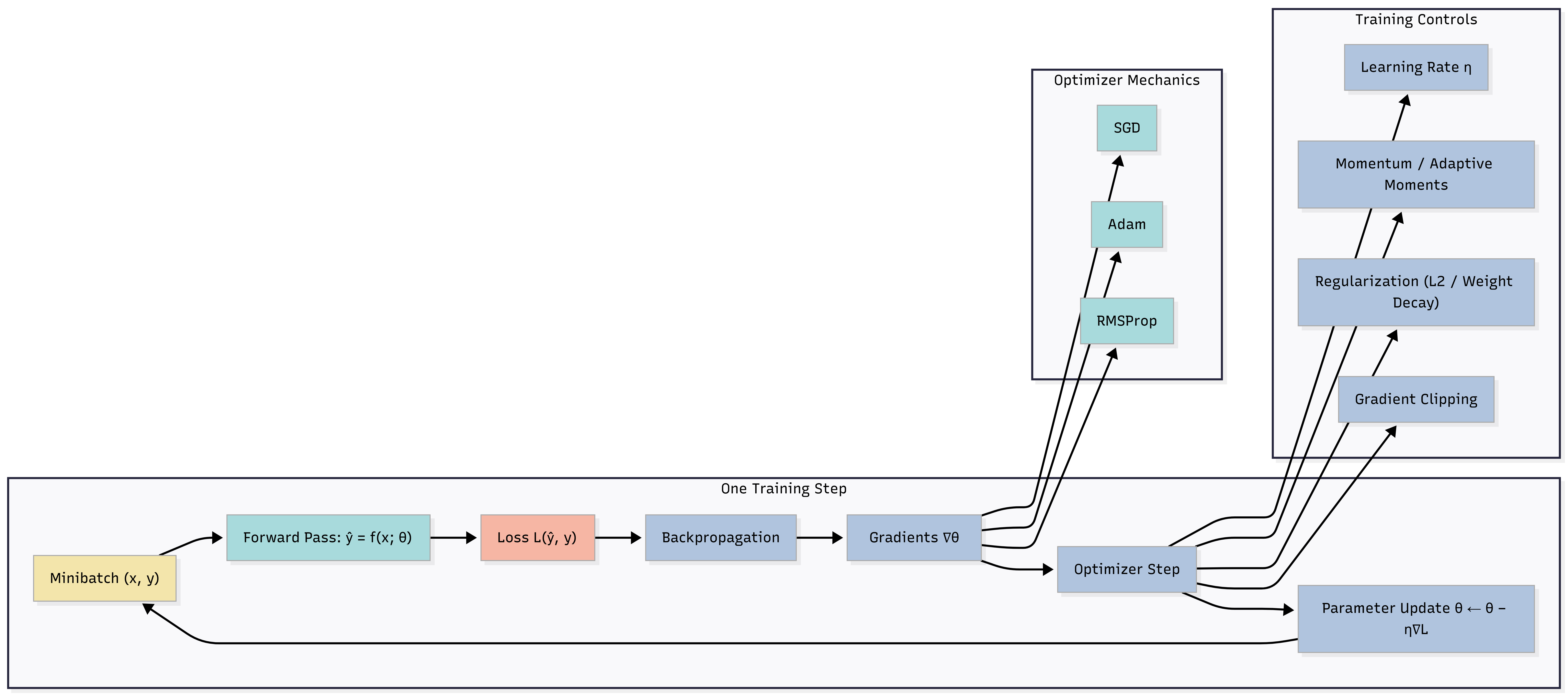
Caption: Forward → Loss → Backprop → Optimizer uses ∇L to update θ. Optimizer mechanics (SGD, Adam, RMSProp) and training controls (learning rate η, momentum, regularization, gradient clipping) feed into the optimizer step. The loop returns to the next minibatch.

---

10. FAQs & Common Student Struggles

Q1. What is the learning rate?

The learning rate (η) is the step size in the update: how much we move the parameters in the direction of −∇L (or the optimizer’s direction). Too high → instability; too low → slow training.

---

Q2. What is learning rate decay?

Learning rate decay (or scheduling) means reducing η over time (e.g., after each epoch or following a cosine curve). Early training often benefits from a larger η; later, a smaller η helps fine-tune and converge stably.

---

Q3. What is warmup?

Warmup is increasing the learning rate from 0 (or a small value) to the target value over the first few steps or epochs. It avoids huge updates when optimizer state (e.g., Adam’s m, v) is still initializing. Common in Transformers and large-batch training.

---

Q4. Is Adam always better than SGD?

No. Adam often converges faster and is easier to tune (less sensitive to η). But in some settings (e.g., certain CNN benchmarks), SGD with momentum and a good LR schedule can achieve better generalization. So: Adam for speed and ease; SGD (+ momentum) when you want to squeeze the best test performance and are willing to tune.

Interview tip: Say “Adam is often the default for fast convergence; SGD with momentum can generalize better in some vision tasks and is worth trying when tuning for final accuracy.”

---

Q5. What is momentum?

Momentum is a running average of past gradients. Instead of updating with only the current gradient, we use a weighted sum of current and previous gradients. It smooths updates and can help cross flat regions and escape saddle points.

---

Q6. What is bias correction in Adam?

Adam’s m and v start at 0, so early estimates are biased toward 0. Bias correction divides m by (1−β₁^t) and v by (1−β₂^t) so that the effective momentum and scale are correct from the first steps.

---

Q7. What is the difference between weight decay and L2 regularization?

L2 regularization adds a penalty to the loss (e.g., λ‖θ‖²) and is included in the gradient, so it gets scaled by the optimizer (e.g., in Adam, by 1/√v). Weight decay (especially decoupled, as in AdamW) applies a direct shrinkage θ ← θ − λθ (or similar) separately from the gradient update. For Adam, decoupled weight decay (AdamW) often generalizes better than L2 in the loss.

---

Q8. How do I choose batch size and learning rate?

Batch size: Larger → more stable gradients but fewer steps per epoch and higher memory. Learning rate: Often increased when batch size is larger (e.g., linear scaling rule: double batch size ⇒ double η, up to a point). Tune with validation performance; use warmup for large batches.

---

Q9. What does “adaptive” mean in Adam?

Adaptive means the effective step size is different per parameter (or per dimension). Parameters with large historical gradients get smaller steps (divided by √v); parameters with small gradients get relatively larger steps. So the optimizer adapts to the geometry of the loss.

---

Q10. Why does SGD sometimes generalize better than Adam?

Not fully settled; possible factors: noisier updates (SGD) may act as implicit regularization; Adam’s adaptive scaling might converge to sharper minima in some settings; weight decay interaction (AdamW helps). In practice: try both when aiming for best generalization.

---

11. Applications (With How They Are Achieved)

1. Training Any Neural Network

Application: Image classification, NLP, recommendation, etc.

How optimizers achieve this: Every training step ends with an optimizer update: backprop gives ∇L(θ), the optimizer computes θ_new. Without an optimizer, parameters would never change and the model would not learn.

Example: Training BERT: AdamW with warmup and linear decay; each step updates millions of parameters using gradients from backprop.

---

2. Fast Prototyping and Research

Application: Quick experiments, hyperparameter search.

How optimizers achieve this: Adam (or AdamW) with a default learning rate (e.g., 1e-3 or 3e-4) often works “out of the box,” so researchers can iterate quickly. SGD usually needs more tuning (η, momentum, schedule).

Example: Trying a new architecture: start with Adam and a cosine schedule; switch to SGD + momentum if targeting a benchmark and have time to tune.

---

3. Production Training Pipelines

Application: Training at scale (large batch, distributed).

How optimizers achieve this: Learning rate schedules (warmup + decay) and batch-size–dependent LR (e.g., linear scaling) are part of the optimizer/scheduler choice. AdamW is common for transformer fine-tuning; SGD + momentum for some vision pipelines.

Example: Fine-tuning a vision transformer: AdamW, batch size 256, warmup for 5% of steps, then cosine decay to 0.

---

4. Sparse and Imbalanced Updates

Application: Embeddings, sparse features.

How optimizers achieve this: Adaptive optimizers (AdaGrad, Adam) give smaller steps to parameters that get large gradients often, and relatively larger steps to rarely updated parameters. So sparse dimensions still get meaningful updates.

Example: Word embeddings: parameters for rare words get fewer updates; Adam’s per-parameter scaling can help them learn effectively.

---

12. Advantages and Limitations (With Examples)

Advantages

1. Systematic improvement
Optimizers give a repeatable rule to reduce the loss; we don’t guess parameter changes by hand.

Example: Training a 100M-parameter model by hand would be impossible; SGD/Adam automate updates for all parameters.

---

2. Faster and more stable convergence
Momentum and adaptive methods (Adam) often converge faster and are less sensitive to learning rate than vanilla SGD.

Example: Same architecture: with Adam, good validation loss in 10 epochs; with vanilla SGD, might need 50 epochs and careful LR tuning.

---

3. Flexibility
We can choose optimizer and schedule to match the task (e.g., AdamW for Transformers, SGD for some CNNs).

Example: BERT fine-tuning typically uses AdamW; ResNet on ImageNet often uses SGD with momentum and step decay.

---

Limitations

1. Hyperparameter sensitivity
Learning rate (and for Adam, β₁, β₂, weight decay) still need tuning; “default” values don’t always generalize across tasks.

Example: Same Adam default (1e-3) may work for one dataset and diverge or overfit on another.

---

2. Memory and compute cost
Adaptive optimizers (Adam, AdamW) store two extra states per parameter (m, v), increasing memory. Extra computations (bias correction, sqrt) add a bit of compute.

Example: Training a 1B-parameter model with Adam needs roughly 3× parameter-sized tensors (θ, m, v); SGD with momentum needs 2× (θ, m).

---

3. No guarantee of global minimum
Optimizers only drive the loss downward; in non-convex settings they can still get stuck in local minima or saddle points (though momentum and stochasticity help).

Example: Bad initialization or unlucky seed can lead to worse final loss despite using Adam.

---

13. Interview-Oriented Key Takeaways

• An optimizer is the update rule that turns gradients ∇L(θ) into parameter updates; backprop computes ∇L, the optimizer applies the rule.
• SGD: θ ← θ − η∇L (optionally with momentum). Adam: momentum (m) + adaptive scale (v) + bias correction; often default for fast convergence.
• AdamW = Adam + decoupled weight decay; preferred when using weight decay (e.g., BERT, ViT).
• Learning rate = step size; schedules (warmup, decay, cosine) improve stability and convergence.
• Adam is usually easier to tune and converges fast; SGD with momentum can generalize better in some vision settings—choose by task and tuning budget.
• Momentum smooths updates and helps escape saddle points; adaptive methods scale step size per parameter.

---

14. Common Interview Traps

Trap 1: “Is Adam always better than SGD?”

❌ Wrong: Yes, Adam is always better.

✅ Correct: Adam often converges faster and is easier to tune, but SGD with momentum (and a good LR schedule) can achieve better generalization in some settings (e.g., certain CNNs). Use Adam for speed and ease; consider SGD when optimizing for best test accuracy.

---

Trap 2: “Backpropagation updates the weights.”

❌ Wrong: Backprop updates the weights.

✅ Correct: Backpropagation only computes the gradients ∂L/∂θ. The optimizer (SGD, Adam, etc.) updates the weights using those gradients. Backprop = gradient computation; optimizer = parameter update.

---

Trap 3: “Learning rate should be constant throughout training.”

❌ Wrong: One learning rate for the whole training.

✅ Correct: Many recipes use schedules: e.g., warmup (ramp up η at the start) and decay (reduce η over time, e.g., cosine). Constant η is fine for quick experiments but often suboptimal for final performance.

---

Trap 4: “Weight decay and L2 regularization are the same in Adam.”

❌ Wrong: They are the same.

✅ Correct: In Adam, L2 in the loss gets scaled by the adaptive learning rate (1/√v). AdamW uses decoupled weight decay (separate from the gradient update), which often generalizes better. So in practice we prefer AdamW with weight decay over Adam with L2 in the loss.

---

Trap 5: “Momentum is the same as the learning rate.”

❌ Wrong: Momentum is just another name for learning rate.

✅ Correct: Learning rate (η) is the step size. Momentum is a running average of past gradients (smoothing). They are different: we have both η and momentum coefficient β (e.g., 0.9).

---

Trap 6: “Bigger batch size always means faster training.”

❌ Wrong: Just increase batch size to train faster.

✅ Correct: Larger batch ⇒ fewer steps per epoch (same amount of data). We may need to adjust learning rate (e.g., linear scaling) or train more epochs to get similar optimization behavior. Also, very large batches can sometimes generalize slightly worse (we may need LR warmup or tuning).

---

15. Simple Real-Life Analogy

Gradient is like the slope under your feet. Optimizer is your walking policy: SGD is “take a fixed-size step downhill”; momentum is “keep some inertia so you don’t stop at every small bump”; Adam is “take bigger steps where it’s been flat and smaller steps where it’s been steep.” Learning rate is how big your default step is; warmup is “start with small steps until you get your bearings.”

---

16. Optimizers in System Design – Interview Traps

Trap 1: One Optimizer for All Stages (Pretrain vs Fine-Tune)

Wrong thinking: Use the same optimizer and learning rate for pretraining and fine-tuning.

Correct thinking: Pretraining often uses large batch, long schedule, and Adam/AdamW with warmup + decay. Fine-tuning may use smaller LR, fewer steps, and sometimes different schedule (e.g., linear decay over few epochs). Match optimizer and schedule to the phase.

Example: BERT pretraining: AdamW, warmup, long decay. BERT fine-tuning on a task: AdamW with smaller LR (e.g., 2e-5), short linear decay.

---

Trap 2: Ignoring Batch Size When Comparing Runs

Wrong thinking: “I doubled batch size, so I’ll finish in half the time with the same result.”

Correct thinking: Steps per epoch = dataset size / batch size. Doubling batch size halves steps per epoch. To keep optimization similar, often scale learning rate (e.g., linear scaling) or train more epochs. Otherwise, same “number of epochs” means fewer total updates and possibly worse convergence.

Example: Batch 32, 10 epochs, η=0.01. If you switch to batch 64, try η=0.02 and still 10 epochs, or keep η and train 20 epochs.

---

Trap 3: Optimizing Only Training Loss

Wrong thinking: “Optimizer’s job is to minimize training loss; that’s enough.”

Correct thinking: The goal is good validation/test performance and generalization. Aggressive optimization (e.g., very high LR, no weight decay) can reduce training loss but hurt generalization. Use validation metrics and regularization (weight decay, dropout) together with optimizer choice.

Example: Adam with no weight decay might overfit; AdamW with appropriate weight decay often generalizes better.

---

17. Interview Gold Line

Optimizers are the rule that turns gradients into parameter updates; choosing the right one (SGD vs Adam, schedule, weight decay) is a key lever for both convergence speed and generalization.

---

18. Self-Check and “Think About It” Prompts

Self-check 1: What is the difference between backpropagation and the optimizer? Who actually changes the weights?

Self-check 2: In one sentence each, what do momentum and adaptive learning rate (e.g., in Adam) do?

Think about it: If you switch from Adam to SGD with momentum for the same model, what hyperparameters would you expect to tune more carefully?

Self-check answers (concise):
- 1: Backprop computes ∂L/∂θ; the optimizer uses those gradients to update θ. The optimizer changes the weights; backprop does not.
- 2: Momentum = running average of gradients (smoothing). Adaptive LR = per-parameter step size (e.g., scale by 1/√v in Adam).
- 3: Learning rate and schedule (SGD is more sensitive); possibly momentum coefficient β; and often more epochs or careful decay.

---

19. Likely Interview Questions

• What is an optimizer and how does it differ from backpropagation?
• Write the update rule for SGD and for Adam (including bias correction).
• What is learning rate warmup and why is it used?
• Is Adam always better than SGD? When would you use each?
• What is AdamW and how does it differ from Adam?
• What is momentum? Why does it help?
• How does batch size affect the choice of learning rate?

---

20. Elevator Pitch

30 seconds:
An optimizer is the algorithm that updates the model parameters using the gradients. Backprop computes the gradients; the optimizer applies a rule like θ ← θ − η∇L (SGD) or the Adam update (momentum + adaptive scaling). Learning rate controls step size; schedules like warmup and decay improve stability. Adam is often the default for fast convergence; SGD with momentum can generalize better in some vision tasks.

2 minutes:
Optimizers take the gradients from backpropagation and produce the actual parameter updates. Vanilla SGD is θ ← θ − η∇L. SGD with momentum keeps a running average of gradients to smooth updates and help escape saddle points. Adam combines momentum with per-parameter adaptive scaling (using second moments) and bias correction, so it’s robust to learning rate and converges quickly. AdamW adds decoupled weight decay, which often generalizes better than L2 in the loss. Learning rate schedules—warmup, then decay (e.g., cosine)—are standard in modern training. Adam is the default for many NLP and transformer models; SGD with momentum is still preferred in some vision benchmarks when tuning for best generalization. Backprop only computes gradients; the optimizer is what actually updates the weights.

---

21. One-Page Cheat Sheet (Quick Revision)

Concept	Definition / formula
Optimizer	Algorithm that updates θ using ∇L(θ); backprop computes ∇L, optimizer applies the rule.
SGD	θ ← θ − η ∇L(θ) (per minibatch).
SGD + momentum	m ← βm + ∇L; θ ← θ − η·m.
Adam	m, v = first and second moment; bias-correct m̂, v̂; θ ← θ − η·m̂/(√v̂+ε).
AdamW	Adam + decoupled weight decay (not in gradient).
Learning rate η	Step size; how much we move in the descent direction.
Warmup	Ramp η from 0 (or small) to target in early steps.
Weight decay	Shrink parameters (e.g., θ ← θ − λθ); in AdamW, decoupled from gradient.
Steps per epoch	(Dataset size) / (Batch size).
Backprop vs optimizer	Backprop computes ∇L; optimizer updates θ using ∇L.

---

22. Formula Card

Name	Formula / statement
Vanilla SGD	θ ← θ − η ∇L(θ)
SGD + momentum	m ← β·m + ∇L(θ); θ ← θ − η·m
Adam (concept)	m ← β₁·m + (1−β₁)·∇L; v ← β₂·v + (1−β₂)·(∇L)²; m̂ = m/(1−β₁^t); v̂ = v/(1−β₂^t); θ ← θ − η·m̂/(√v̂+ε)
Steps per epoch	(Dataset size) / (Batch size)
Total steps	Epochs × Steps per epoch

---

23. What’s Next and Revision Checklist

What’s Next

• Regularization and Generalization: Dropout, BatchNorm, L1/L2, weight decay. Optimizers interact with these (e.g., AdamW + weight decay).
• Hyperparameter Tuning: Learning rate search, batch size, schedule length. Builds on optimizer and schedule concepts.
• Training Dynamics: Loss curves, convergence, debugging (e.g., loss not decreasing → LR or optimizer choice).

Revision Checklist

Before an interview, ensure you can:

1. Define an optimizer (update rule that uses ∇L to produce θ_new).
2. Write the update for SGD and the idea of Adam (momentum + adaptive + bias correction).
3. Compare SGD vs Adam (when to use each; generalization vs speed).
4. Explain warmup and learning rate decay (why and when).
5. State the difference between backprop and optimizer (compute ∇L vs update θ).
6. Correct the trap: “Adam is always better” (no; SGD can generalize better in some cases).
7. Explain AdamW (Adam + decoupled weight decay).

Related Topics

• Optimization Fundamentals (gradient descent, convex vs non-convex)
• Backpropagation (how ∇L is computed)
• Loss Functions (what we minimize)
• Regularization (weight decay, dropout—interact with optimizers)

---

End of Optimizers study notes.