Pre-Notes: Learning Objectives & Prerequisites

Learning Objectives

By the end of this note you will be able to:

• Define optimization in the context of ML/DL and distinguish it from “just minimizing loss.”
• Explain convex vs non-convex loss surfaces and why deep learning uses non-convex optimization.
• Describe saddle points, local minima, and global minima and how they affect training.
• Justify why deep learning works despite non-convexity (e.g., loss landscape structure, wide minima).
• Connect gradient descent to maximum likelihood estimation (MLE) when using common loss functions.
• Use correct terminology in interviews (e.g., “we optimize the parameters” vs “we minimize the loss”).

Prerequisites

Before starting, you should know:

• Basic calculus: partial derivatives, chain rule, gradient as a vector of partials.
• Loss function: what it measures (e.g., MSE, cross-entropy) and that training aims to reduce it.
• Weights/parameters: that a neural network has learnable parameters we update during training.

If you don’t, review Calculus for Deep Learning and the Loss Functions topic first.

Where This Fits

• Builds on: Calculus (gradients, chain rule), Loss Functions (what we minimize).
• Needed for: Optimizers (SGD, Adam, learning rate schedules), Backpropagation (which produces the gradients optimization uses).

This topic is part of Phase 1: Mathematical Foundations and feeds directly into Optimizers and Backpropagation.

---

1. What is Optimization?

Optimization in machine learning and deep learning is the process of finding parameter values (e.g., weights) that minimize a loss function (or maximize a reward/metric) on the data.

In simple words: we have a loss that tells us how wrong the model is; optimization is the set of methods we use to change the parameters so that this loss gets smaller (or the metric gets better).

Simple Intuition

Imagine you are on a hilly landscape in the fog and want to reach the lowest valley (minimum height). You can’t see the whole map; you can only feel the slope under your feet. You take small steps downhill. That process—using local information (slope/gradient) to move toward a minimum—is the core idea of gradient-based optimization.

Formal Definition (Interview-Ready)

Optimization (in ML/DL) is the iterative process of updating model parameters (e.g., weights θ) to minimize a scalar objective L(θ) (usually the loss), using information from the gradient (and sometimes higher-order or momentum terms) to decide the direction and size of each update.

---

In a Nutshell

Optimization = choosing how to move the parameters so the loss decreases. In practice we use gradient-based methods: compute ∇L(θ) and take a step in the direction that reduces L.

---

2. Why Do We Need Optimization?

Training a model means adjusting its parameters so predictions match targets. Without a systematic way to do this, we could not train neural networks at scale.

Old vs New Paradigm

Paradigm	Role of optimization
Hand-crafted rules	No learning; no optimization of parameters
Classical ML	Optimize a small set of parameters (e.g., SVM)
Deep Learning	Optimize millions/billions of parameters

Key Reasons

• The loss function tells us how bad the current parameters are; optimization is the only way to improve them.
• Gradient-based optimization scales to huge parameter counts because we only need first-order (gradient) information per step.
• Understanding optimization helps you choose optimizers, learning rates, and schedules and debug training (e.g., stuck in saddle points, bad local minima).

Real-World Relevance

Domain	Why optimization matters
Training NNs	Every training step is an optimization step (update weights).
Hyperparameter tuning	Learning rate, batch size, etc. affect the optimization trajectory.
Research	New optimizers (Adam, AdamW, Lion) improve convergence.

---

3. Core Building Block: What We Optimize and How

What We Optimize

• Variables: Model parameters θ (weights, biases).
• Objective: A scalar L(θ) — in DL usually the loss (e.g., cross-entropy, MSE) on the training (or minibatch) data.

We want: θ* such that L(θ*) ≤ L(θ) for all θ (global minimum). In practice we only ever search for good local minima or low-loss regions.

How We Optimize (Gradient-Based Methods)

The core mechanism is:

1. Compute the gradient ∇L(θ) (via backpropagation).
2. Take a step in the direction that decreases L (e.g., −∇L(θ)).
3. Repeat until convergence or a fixed number of steps.

Update rule (vanilla gradient descent):

θ_new = θ_old − η · ∇L(θ_old)

where η is the learning rate.

Gradient points in the direction of steepest ascent. So −∇L(θ) points in the direction of steepest descent; moving a small step in that direction reduces the loss (for small enough step size).

---

In a Nutshell

The core building block is gradient descent: compute ∇L(θ), then θ ← θ − η ∇L(θ). All common optimizers (SGD, Adam, etc.) are variants of this idea (e.g., momentum, adaptive step size).

---

Think about it: Why do we use minus the gradient (descent) instead of plus (ascent)? What would happen if we used the gradient direction as-is?

---

4. Convex vs Non-Convex Loss

Convex Loss

• Convex function: For any two points, the line segment between them lies above or on the graph. In 1D: bowl-shaped (single “dip”).
• Convex optimization: Any local minimum is automatically a global minimum. Gradient descent (with a suitable step size) can converge to the global optimum.

Example: Linear regression with MSE loss is convex in the parameters.

Non-Convex Loss

• Non-convex function: Can have many “dips” and “humps.” Multiple local minima, saddle points, and flat regions.
• Non-convex optimization: We can get stuck in local minima or saddle points; there is no guarantee we reach the global minimum.

Deep learning: Neural network loss surfaces are non-convex in the parameter space. Yet we still train them successfully.

Aspect	Convex loss	Non-convex loss (e.g., DL)
Local vs global	Local min = global min	Many local minima, saddle points
Guarantees	Can guarantee global opt	No such guarantee
Typical use	Linear models, some SVMs	Neural networks

Interview-ready: In deep learning we minimize a non-convex loss. We don’t have a guarantee of reaching the global minimum, but in practice gradient-based methods often find good enough minima that generalize well.

---

In a Nutshell

Convex = one “bowl”; local min is global. Non-convex = many hills and valleys; we can get stuck. DL uses non-convex optimization; success comes from landscape structure and good initialization/settings, not from convexity.

---

5. Saddle Points and Local vs Global Minima

Critical Points

A critical point is where the gradient is zero: ∇L(θ) = 0. At such a point we don’t know, from the gradient alone, whether we are at a minimum, maximum, or saddle.

Local Minimum

• Local minimum: A point where L is lower than at all nearby points. Gradient is zero; moving a small step in any direction increases (or doesn’t decrease) the loss.
• Risk: We might get stuck there and never reach a better (global) minimum.

Global Minimum

• Global minimum: The point(s) where L is the smallest over the entire parameter space. This is what we would ideally want.
• In non-convex settings we rarely know if we have reached it; we only observe that loss is low and stable.

Saddle Point

• Saddle point: A critical point where the loss decreases in some directions and increases in others (like a horse’s saddle). Gradient is zero, but it is not a local minimum (or maximum).
• Why it matters: Gradient descent can get “stuck” momentarily (zero gradient), but saddle points are usually unstable: small perturbations or momentum can help escape. In high dimensions, saddle points are much more common than local minima.

Point type	Gradient	Behavior nearby	Typical in DL
Local minimum	0	L increases in all directions	Many; often “good”
Global minimum	0	L is lowest everywhere	Unknown in practice
Saddle point	0	L down in some directions, up in others	Very common in high dims

Interview tip: In high-dimensional loss surfaces (like in deep nets), saddle points are more common than “bad” local minima. Momentum and adaptive optimizers (e.g., Adam) help escape saddle points faster than vanilla gradient descent.

---

In a Nutshell

Local min = low point in a small region. Global min = lowest point overall. Saddle point = flat in some directions, down in others; gradient is zero but we can escape. In DL, saddle points are common; bad local minima are less of a problem than once thought.

---

Self-check: What is the gradient at a local minimum, a global minimum, and a saddle point? Why can gradient descent get stuck at all three, and why might we still escape a saddle point?

---

6. Why Deep Learning Works Despite Non-Convexity

This is a key interview topic. Neural nets have non-convex loss surfaces, yet they train well. Reasons include:

1. Landscape structure: Many local minima in practice have similar loss values; finding any of them often gives good generalization.
2. High dimensionality: In high dimensions, “bad” local minima (much worse than average) are relatively rare; saddle points dominate, and we can escape them.
3. Initialization and regularization: Good initialization (e.g., Xavier, He) and regularization (dropout, weight decay) steer optimization toward wider, flatter minima that tend to generalize better.
4. Stochasticity: Minibatch SGD adds noise, which can help escape shallow local minima and saddle points.
5. Overparameterization: Large networks have many solutions (many good minima); optimization often finds one of them.

Interview-ready: Deep learning works despite non-convexity because the loss landscape in practice has many good local minima with similar loss, saddle points that we can escape (e.g., with momentum), and high dimensionality where worst-case local minima are less dominant. We don’t need the global minimum—we need a good enough minimum that generalizes.

---

In a Nutshell

We don’t need the global minimum. We need a good local minimum in a well-behaved part of the loss surface. Overparameterization, stochasticity, and good initialization make that achievable in practice.

---

7. Gradient Descent as Maximum Likelihood

This connects optimization to statistics and is a common interview angle.

Maximum Likelihood Estimation (MLE)

• We assume data D comes from a model P(D | θ). MLE chooses θ that maximizes the likelihood P(D | θ) (or log-likelihood log P(D | θ)).
• Equivalently, we minimize the negative log-likelihood (NLL).

Link to Loss and Gradient Descent

• For many standard models, the loss function we use in practice is exactly (or proportional to) the negative log-likelihood of the data under the model.
  • Example (regression): MSE loss ↔︎ Gaussian likelihood → minimizing MSE is MLE for a Gaussian output model.
  • Example (classification): Cross-entropy loss ↔︎ categorical (Bernoulli/multinoulli) likelihood → minimizing cross-entropy is MLE for the class probabilities.
• So when we minimize the loss with gradient descent, we are (under that model) performing (stochastic) MLE: we are finding parameters that maximize the likelihood of the training data.

Interview-ready: Minimizing MSE (with a Gaussian output) or cross-entropy (with a probabilistic classification model) is equivalent to maximum likelihood estimation. Gradient descent on that loss is thus an iterative way to do MLE.

---

In a Nutshell

For the usual regression and classification losses (MSE, cross-entropy), minimizing the loss = maximizing the data likelihood. So gradient descent on the loss is doing MLE for the model parameters.

---

8. Process: One Step of Optimization (Recap)

A single optimization step in training looks like this:

1. Forward pass: Compute predictions and loss L for the current minibatch.
2. Backward pass: Compute ∇L(θ) (gradients w.r.t. all parameters).
3. Update: Apply the optimizer rule, e.g. θ ← θ − η ∇L(θ) (or with momentum/adaptive scaling).

This is repeated for many steps (and epochs) until convergence or a budget.

Step	What happens
Forward	Loss L(θ) computed
Backward	Gradients ∇L(θ) computed (backprop)
Update	Parameters θ updated using gradient (and possibly momentum, etc.)

---

9. Comparison: Optimization in Classical ML vs Deep Learning

Aspect	Classical ML (e.g., linear, SVM)	Deep Learning
Loss surface	Often convex	Non-convex
Goal	Global optimum (when convex)	Good local minimum / low loss
Scale	Few parameters	Millions/billions of parameters
Method	Closed form or small-scale GD	Iterative gradient-based (SGD, Adam)
Guarantees	Can have optimality guarantees	No global optimality guarantee

---

10. Key Sub-Topics (Quick Reference)

Sub-topic	One-line summary
Convex vs non-convex	Convex: one global min; non-convex: many local mins/saddles
Saddle points	Zero gradient; escape possible; common in high dimensions
Local vs global minima	Local = best in neighborhood; global = best everywhere
Why DL works (non-convex)	Good minima abound; saddles escapable; overparameterization
GD as MLE	Minimizing NLL loss = MLE; GD implements it iteratively

---

11. FAQs & Common Student Struggles

Q1. What is optimization in one sentence?

Finding parameter values that minimize the loss function (or maximize a performance metric) using iterative, gradient-based updates.

---

Q2. Is “optimization” the same as “minimizing the loss”?

In ML/DL, yes in practice: we almost always minimize a loss. So “we optimize the parameters” and “we minimize the loss” mean the same thing when the objective is the loss. (Technically, optimization can also mean maximizing something, e.g., reward in RL.)

---

Q3. Why is the neural network loss non-convex?

Because the model is non-linear in the parameters (many compositions of non-linear activations and weights). Non-linearity leads to multiple local minima and saddle points in the loss surface.

---

Q4. Can we get stuck at a saddle point forever?

In theory, gradient descent could sit at a saddle (gradient = 0). In practice, numerical noise, minibatch stochasticity, and momentum (or other optimizers) usually allow escape. Saddle points are not stable minima.

---

Q5. Are local minima always bad?

No. Many local minima in deep nets have similar loss and generalize well. “Bad” local minima (much higher loss) are less common in high-dimensional overparameterized networks. We care more about generalization than about being at the global minimum.

---

Q6. What is the difference between local and global minimum?

Local minimum: Loss is lower than at all nearby points. Global minimum: Loss is the smallest over the entire parameter space. In non-convex settings we usually find a local (or near-local) minimum, not necessarily the global one.

---

Q7. How is gradient descent related to maximum likelihood?

For standard losses (e.g., MSE for Gaussian outputs, cross-entropy for classification), minimizing the loss is equivalent to maximizing the likelihood of the data. Gradient descent on that loss is therefore an iterative method for MLE.

---

Q8. Why do we use gradient descent instead of solving ∇L(θ) = 0 directly?

Because in deep learning the system of equations ∇L(θ) = 0 is huge and non-linear; there is no closed-form solution. Gradient descent (and its variants) are scalable iterative methods that only need gradient computation (via backprop) and simple updates.

---

12. Applications (With How They Are Achieved)

Optimization is universal in ML/DL: every trained model uses it. Below are concrete places where understanding optimization fundamentals matters.

1. Training Any Neural Network

Application: Image classification, NLP, recommendation, etc.

How optimization achieves this: We define a loss (e.g., cross-entropy, MSE), compute gradients via backprop, and apply an optimizer (SGD, Adam, etc.) to update weights. Without optimization, no learning.

Example: Training a ResNet for ImageNet: every batch step is an optimization step minimizing cross-entropy.

---

2. Hyperparameter and Learning Rate Tuning

Application: Choosing learning rate, batch size, optimizer.

How optimization fundamentals help: Understanding convex vs non-convex, saddle points, and learning rate effects helps you choose schedules (warmup, decay) and diagnose training (e.g., loss not decreasing → learning rate or saddle).

Example: Using learning rate warmup to avoid large early updates in Transformers.

---

3. Research and New Optimizers

Application: Adam, AdamW, Lion, etc.

How optimization achieves this: New algorithms still follow “gradient + update rule” but change how we use the gradient (momentum, adaptive step sizes, weight decay). Understanding fundamentals (descent direction, step size, curvature) is essential to design and compare them.

Example: AdamW decouples weight decay from the gradient-based update to improve generalization.

---

13. Advantages and Limitations (With Examples)

Advantages

1. Scalable to huge parameter counts
We only need gradients (first-order information) per step, which backprop provides efficiently.

Example: Training GPT-scale models with billions of parameters via gradient-based optimization.

2. Flexible
Same idea (minimize loss, follow gradient) works for many architectures and tasks; we just change the loss and model.

Example: Same optimizer (e.g., Adam) used for CNNs, RNNs, and Transformers.

3. Theoretically and practically well understood
Convergence and stability are studied (e.g., for convex case; for non-convex, empirical success is well documented).

Example: Proofs of convergence for SGD under certain conditions; extensive benchmarks for optimizers.

Limitations

1. No guarantee of global minimum in non-convex case
We might converge to a poor local minimum or get stuck at a saddle (though in practice this is often manageable).

Example: Some random seeds or bad initialization can lead to worse final loss.

2. Sensitive to hyperparameters
Learning rate, batch size, and optimizer choice strongly affect convergence and generalization.

Example: Too high a learning rate can cause divergence; too low can make training very slow.

3. Computational cost
Each step requires a forward and backward pass; for large models and data, optimization is expensive.

Example: Full fine-tuning of a large language model requires significant GPU time and memory.

---

14. Interview-Oriented Key Takeaways

• Optimization = finding parameters that minimize the loss (or maximize a metric) using iterative, gradient-based updates.
• Gradient descent is the core: θ ← θ − η ∇L(θ); all common optimizers are variants (momentum, adaptive step size).
• Convex loss: local min = global min. Non-convex (DL): many local minima and saddle points; we aim for a good local minimum.
• Saddle points (zero gradient, but not a min) are common in high dimensions; momentum and stochasticity help escape.
• Why DL works despite non-convexity: many good minima, saddle-dominated landscape, overparameterization, good initialization.
• Minimizing MSE or cross-entropy (with the right probabilistic model) is MLE; gradient descent on that loss implements MLE iteratively.

---

15. Common Interview Traps

Trap 1: “Is the goal of optimization to find the global minimum?”

Wrong: Yes, we always want the global minimum.

Correct: In deep learning the loss is non-convex; we rarely can find or verify the global minimum. The goal is to find a good local minimum (or low-loss region) that generalizes well.

---

Trap 2: “If the gradient is zero, we have found the minimum.”

Wrong: Yes, gradient zero means we’re done.

Correct: Gradient zero only means a critical point. It could be a local minimum, a local maximum, or a saddle point. We need further checks (e.g., second-order or behavior over time) to know which.

---

Trap 3: “Non-convex optimization is hopeless for neural networks.”

Wrong: Non-convex means we can’t train NNs reliably.

Correct: Non-convex means we don’t have a guarantee of the global minimum. In practice, gradient-based methods find good minima; saddle points are escapable; and overparameterization helps.

---

Trap 4: “Gradient descent and backpropagation are the same thing.”

Wrong: They are the same.

Correct: Backpropagation computes the gradients ∇L(θ). Gradient descent (or another optimizer) uses those gradients to update θ. They work together but are different steps.

---

Trap 5: “Minimizing the loss has nothing to do with statistics.”

Wrong: Loss is just a number we minimize.

Correct: For standard losses (MSE, cross-entropy), minimizing the loss is equivalent to maximum likelihood estimation under the corresponding probabilistic model. So optimization is doing MLE.

---

16. Simple Real-Life Analogy

Optimization is like hiking in the fog to reach the lowest valley: you can’t see the whole map, but you can feel the slope under your feet. You take steps downhill (opposite to the gradient). Convex terrain has one valley (any low point is the lowest). Non-convex terrain has many valleys and saddles; you aim for a low enough valley, not necessarily the single lowest point on the whole map.

---

17. Optimization in System Design – Interview Traps (If Applicable)

Trap 1: Optimizing Training Loss vs Production Metric

Wrong thinking: If training loss is low, the model is good for production.

Correct thinking: Training loss measures fit to training data. Production depends on distribution shift, latency, and business metrics. Optimize for what you can measure in production (e.g., A/B tests, calibrated metrics).

Example: A model optimized only for cross-entropy might have poor calibration or high false-positive rate in the wild.

---

Trap 2: One Learning Rate for All Stages

Wrong thinking: Pick one learning rate and use it for the whole training.

Correct thinking: Many pipelines use warmup and decay (or cosine schedule). Early and late training may need different learning rates for stability and fine convergence.

Example: Transformers often use warmup to avoid instability in the first steps.

---

Trap 3: Ignoring Batch Size When Comparing Runs

Wrong thinking: Same “epochs” means same optimization.

Correct thinking: Number of optimization steps = (epochs × dataset size) / batch size. Larger batch size ⇒ fewer steps per epoch. You may need to scale learning rate or epochs when changing batch size.

Example: Doubling batch size often requires adjusting learning rate (e.g., linear scaling rule) or training longer.

---

18. Interview Gold Line

Optimization in deep learning is not about finding the global minimum—it’s about finding a good enough minimum, efficiently and reliably, so the model generalizes.

---

19. Visual: Optimization Landscape (Conceptual)

Below is a conceptual view of convex vs non-convex and critical points. Use it to anchor terms like local/global minimum and saddle point.

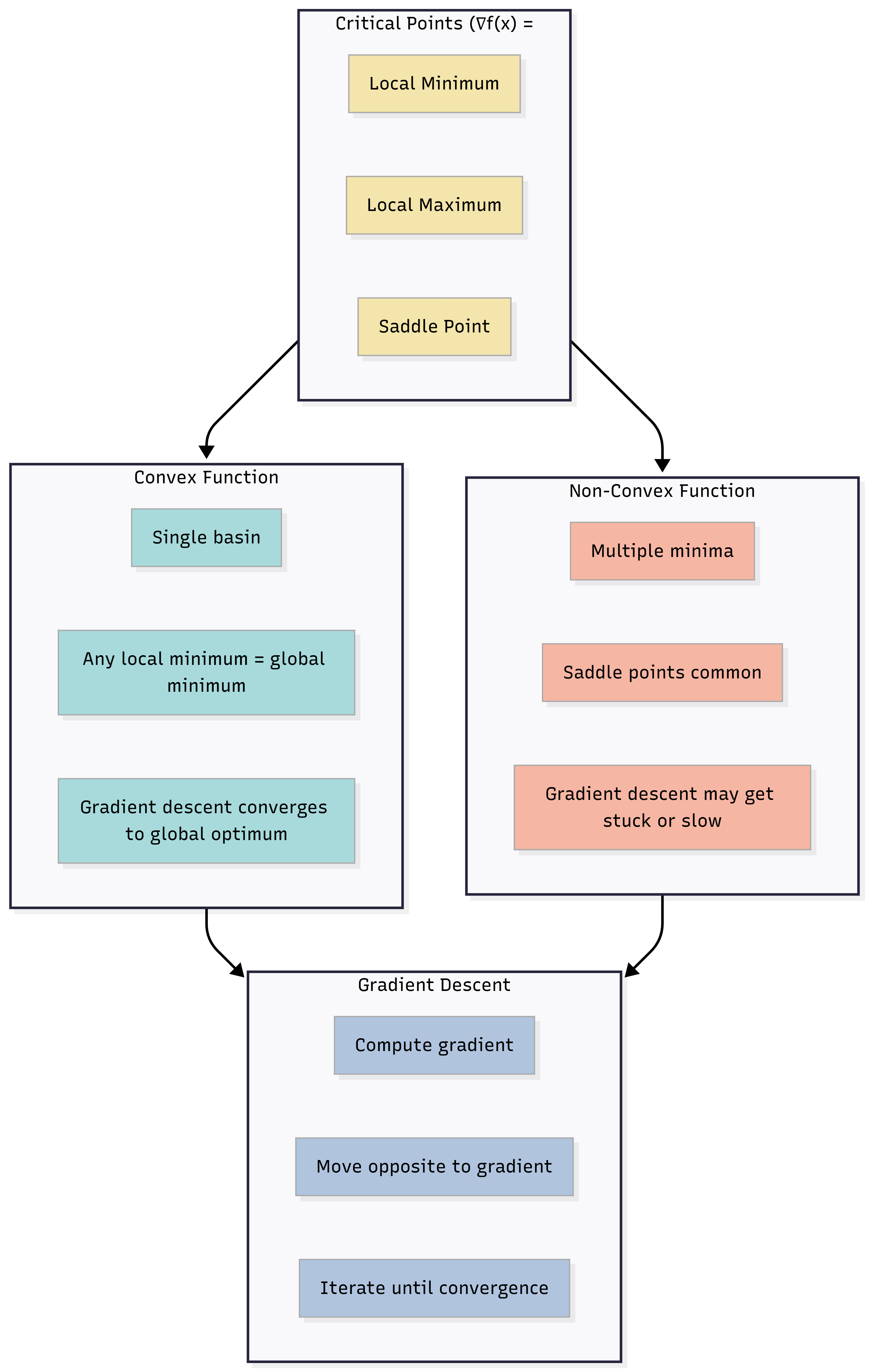
Caption: In a convex setting, one valley (local = global). In a non-convex setting, many valleys and saddles; gradient descent follows the local slope (gradient) toward a nearby low point.

---

20. Self-Check and “Think About It” Prompts

Self-check 1: What is the difference between a local minimum and a saddle point? Why might gradient descent escape a saddle but stay at a local minimum?

Self-check 2: For regression with Gaussian noise, what is the relationship between minimizing MSE and maximum likelihood?

Think about it: If you double the batch size, how might you need to change the learning rate or number of epochs to keep optimization behavior similar?

Self-check answers (concise):
- 1: At both, ∇L = 0. At a local minimum, L increases in all directions; at a saddle, L decreases in some directions. So a small step in a descent direction reduces L at a saddle, allowing escape; at a true local minimum no such direction exists.
- 2: Under a Gaussian noise model, the negative log-likelihood is proportional to MSE; so minimizing MSE = maximizing likelihood.
- 3: Often increase learning rate (e.g., linear scaling with batch size) or train for more epochs so total number of updates is similar.

---

21. Likely Interview Questions

• What is optimization in the context of deep learning?
• Explain convex vs non-convex loss. Why is the NN loss non-convex?
• What is a saddle point? How is it different from a local minimum?
• Why does deep learning work even though the loss is non-convex?
• How is gradient descent related to maximum likelihood estimation?
• What is the difference between backpropagation and gradient descent?
• What happens when the gradient is zero? Are we necessarily at a minimum?

---

22. Elevator Pitch

30 seconds:
Optimization is the process of finding model parameters that minimize the loss. We do it iteratively: compute the gradient of the loss with respect to the parameters (via backprop), then take a step in the opposite direction (gradient descent). Neural network loss is non-convex, so we don’t guarantee the global minimum, but in practice we find good local minima that generalize well.

2 minutes:
Optimization in deep learning means minimizing a loss function over the model’s parameters. The core idea is gradient descent: the gradient points uphill, so we update parameters in the opposite direction to go downhill. The loss surface for neural networks is non-convex—it has many local minima and saddle points—so we can’t guarantee finding the global minimum. Still, deep learning works because there are many good local minima with similar loss, saddle points can be escaped with momentum or stochasticity, and overparameterization helps. For standard losses like MSE and cross-entropy, minimizing the loss is equivalent to maximum likelihood estimation, so gradient descent is effectively doing MLE. Backpropagation computes the gradients; the optimizer (SGD, Adam, etc.) uses them to update the weights.

---

23. One-Page Cheat Sheet (Quick Revision)

Concept	Definition / formula
Optimization	Finding θ that minimizes L(θ) using iterative updates.
Gradient descent	θ ← θ − η ∇L(θ).
Convex	One global min; local min = global min.
Non-convex	Many local minima, saddle points; no global guarantee.
Local minimum	L(θ) ≤ L(θ’) for all θ’ near θ.
Global minimum	L(θ) ≤ L(θ’) for all θ’.
Saddle point	∇L = 0; L decreases in some directions, increases in others.
Why DL works (non-convex)	Many good minima; saddles escapable; overparameterization.
GD as MLE	Minimizing NLL (MSE, cross-entropy) = MLE; GD implements it.
Backprop vs optimizer	Backprop computes ∇L; optimizer uses ∇L to update θ.

---

24. Formula Card

Name	Formula / statement
Gradient descent update	θ ← θ − η ∇L(θ)
Critical point	∇L(θ) = 0
Steepest descent direction	−∇L(θ)
MLE (minimization form)	θ* = argmin_θ −log P(D|θ) = argmin_θ L(θ) when L = NLL
Steps per epoch	(Dataset size) / (Batch size)

---

25. What’s Next and Revision Checklist

What’s Next

• Optimizers (Beyond Adam): SGD, momentum, RMSProp, Adam, AdamW, learning rate schedules, warmup. You’ll use the same optimization fundamentals (gradient, step direction, step size) to compare these algorithms.
• Backpropagation: How ∇L(θ) is computed efficiently; chain rule and computational graphs. Optimization consumes these gradients.
• Loss Functions: MSE, cross-entropy, and why they correspond to MLE. This completes the “what we minimize” side of optimization.

Revision Checklist

Before an interview, ensure you can:

1. Define optimization in one sentence (minimize loss by updating parameters using gradients).
2. Compare convex vs non-convex loss (one valley vs many; local vs global min).
3. Explain saddle point vs local minimum (both have ∇L = 0; saddle is not a min).
4. Justify why deep learning works despite non-convexity (good minima, saddles, overparameterization).
5. State the link between gradient descent and MLE (minimize NLL ⇒ MLE).
6. Correct the trap: “gradient zero ⇒ we’re at the minimum” (could be saddle).
7. Distinguish backpropagation (gradient computation) from gradient descent (parameter update).

Related Topics

• Calculus for Deep Learning (gradients, chain rule)
• Loss Functions (what we minimize)
• Optimizers (SGD, Adam, schedules)
• Backpropagation (how we get ∇L)

---

End of Optimization Fundamentals study notes.