Pre-Notes: Learning Objectives & Prerequisites

Learning Objectives

By the end of this note you will be able to:

• Define derivative, partial derivative, gradient, and chain rule and explain their role in training neural networks.
• Explain why the gradient points in the direction of steepest ascent and how gradient descent uses this to minimize loss.
• Apply the chain rule (multivariable) to simple computational graphs and relate it to backpropagation.
• Distinguish derivative vs gradient vs Jacobian and when each is used in DL.
• Answer common interview questions on calculus in deep learning with correct, concise answers and avoid standard traps.

Prerequisites

You should know…	If you don’t…
Basic algebra (variables, equations, functions)	Review high-school algebra
Idea of “slope” and “rate of change”	Think of speed = rate of change of distance
High-level idea of “learning from data”	Skim Deep Learning from Scratch intro
Vectors and matrices (optional but helpful)	See Linear Algebra for Deep Learning

Where this fits: This topic is part of Phase 1: Mathematical Foundations. It builds on Linear Algebra and basic algebra and is needed for Backpropagation, Optimizers, Loss Functions, and every training loop in deep learning.

---

1. What is Calculus (in the Context of Deep Learning)?

Calculus is the branch of mathematics that studies rates of change (derivatives) and accumulation (integrals). In deep learning, we care almost entirely about derivatives: how a small change in an input or a weight affects the loss. That “sensitivity” is exactly what we use to update weights so the loss goes down.

In simple terms: calculus tells us which way to nudge each parameter to reduce the error—and by how much. Without it, we would have no principled way to train neural networks.

Simple Intuition

Think of standing on a hillside in the fog. You want to get down to the valley (minimum). You can only feel the slope under your feet. Calculus gives you that slope: the gradient tells you the direction of steepest ascent. So you take a step in the opposite direction (steepest descent) and repeat. That’s gradient descent—and it’s how neural networks learn.

Formal Definition (Interview-Ready)

In deep learning, calculus provides the tools—derivatives, partial derivatives, gradients, and the chain rule—to compute how the loss changes with respect to every weight. These derivatives are used by gradient descent (and its variants) to minimize the loss and train the network.

---

2. Why Do We Need Calculus for Deep Learning?

Training a neural network means minimizing a loss function \( L \) that depends on millions of parameters (weights and biases). We need to know:

• In which direction to change each weight so that \( L \) decreases.
• By how much to change it (step size, modulated by learning rate).

Calculus answers both: the gradient of \( L \) with respect to the weights gives the direction of steepest increase; we move in the opposite direction to decrease \( L \).

Key Reasons

Reason	Role in DL
Direction of update	Gradient points “uphill”; we go opposite to go “downhill” (minimize loss).
Efficient learning	One gradient computation tells us how to adjust all parameters at once.
Backpropagation	Chain rule breaks the derivative of the whole network into derivatives of each layer.
Optimizer design	Momentum, Adam, etc. all use gradients (and sometimes second-order info) to decide updates.

Where Calculus Shows Up in DL

DL concept	Calculus used
Gradient descent	Gradient of loss w.r.t. weights
Backpropagation	Chain rule to get gradients layer by layer
Learning rate	Step size along the (negative) gradient direction
Gradient clipping	Magnitude of gradient (norm)
Second-order methods (optional)	Hessian (second derivatives) for curvature

---

3. Core Building Block: Derivative, Partial Derivative, Gradient, Chain Rule

Derivative (Single Variable)

The derivative of a function \( f(x) \) with respect to \( x \) is the rate of change of \( f \) as \( x \) changes:

\[ f'(x) = \frac{df}{dx} = \lim_{h \to 0} \frac{f(x+h) - f(x)}{h} \]

• Interpretation: Slope of the tangent line at \( x \); “how much does \( f \) change if we nudge \( x \) slightly?”
• In DL: When loss \( L \) depends on a single weight \( w \), \( \frac{dL}{dw} \) tells us how to change \( w \) to decrease \( L \) (move \( w \) in the direction of \( -\frac{dL}{dw} \)).

Partial Derivative (Multivariable)

When a function depends on many variables (e.g., \( L(w_1, w_2, \ldots, w_n) \)), the partial derivative \( \frac{\partial L}{\partial w_i} \) is the derivative of \( L \) with respect to \( w_i \) while keeping all other variables fixed.

• In DL: Loss depends on all weights. \( \frac{\partial L}{\partial w_i} \) answers: “If I change only \( w_i \) a little, how does \( L \) change?”

Gradient (Vector of Partials)

The gradient of a scalar function \( f(\mathbf{x}) \) with respect to a vector \( \mathbf{x} = (x_1, \ldots, x_n) \) is the vector of partial derivatives:

\[ \nabla f = \left( \frac{\partial f}{\partial x_1}, \frac{\partial f}{\partial x_2}, \ldots, \frac{\partial f}{\partial x_n} \right)^T \]

• Key fact: The gradient points in the direction of steepest ascent (greatest increase of \( f \)).
• Therefore: To minimize \( f \) (e.g., loss), we take a step in the direction of \( -\nabla f \) (steepest descent).

Interview-ready: The gradient of the loss with respect to the weights is a vector whose \( i \)-th component is “how much the loss changes if we increase the \( i \)-th weight slightly.” We update weights by moving in the opposite direction (gradient descent).

Chain Rule (Multivariable)

When a quantity depends on others in a chain (e.g., loss \( L \) depends on output \( y \), which depends on hidden \( h \), which depends on weights \( \mathbf{w} \)), the chain rule says:

\[ \frac{\partial L}{\partial w} = \frac{\partial L}{\partial y} \cdot \frac{\partial y}{\partial h} \cdot \frac{\partial h}{\partial w} \]

In words: multiply the derivatives along the path from \( L \) back to \( w \). This is exactly what backpropagation does: it propagates the “error signal” backward, multiplying by local derivatives at each layer.

Interview tip: Backpropagation is the chain rule applied to the computational graph of the neural network. Each layer contributes a factor to the product.

In a Nutshell

Core idea: The gradient of the loss w.r.t. weights tells us “which way is up.” We take steps in the opposite direction to minimize the loss. The chain rule lets us compute this gradient efficiently by breaking the network into layers and propagating derivatives backward.

---

Think About It

Before moving on: If the gradient at a weight is zero, what does that tell you about the loss surface at that point? What would gradient descent do there?

Short answer: A zero gradient means we’re at a stationary point (flat in all directions)—could be a local min, local max, or saddle point. Gradient descent would not move (update = \( w - \alpha \cdot 0 = w \)). In practice we might escape due to numerical noise, mini-batch variation (SGD), or momentum.

---

4. Process: From Loss to Weight Update (Gradient Descent)

A compact “process” view of how calculus is used in training:

1. Forward pass: Compute loss \( L \) from inputs and current weights (no calculus yet, just evaluation).
2. Backward pass (backprop): Use the chain rule to compute \( \frac{\partial L}{\partial w} \) for every weight \( w \). This is the gradient of \( L \) w.r.t. all weights.
3. Update: For each weight, \( w \leftarrow w - \alpha \cdot \frac{\partial L}{\partial w} \), where \( \alpha \) is the learning rate.
4. Repeat for many steps (epochs/batches) until the loss is acceptably low.

Gradient Descent in One Formula

\[ \mathbf{w}_{\text{new}} = \mathbf{w}_{\text{old}} - \alpha \cdot \nabla_{\mathbf{w}} L \]

• \( \nabla_{\mathbf{w}} L \): gradient of loss w.r.t. weights.
• \( \alpha \): learning rate (step size).

Why “Steepest” Descent?

The directional derivative of \( f \) in direction \( \mathbf{v} \) (unit vector) is \( \nabla f \cdot \mathbf{v} \). This is maximized when \( \mathbf{v} \) points in the direction of \( \nabla f \). So \( \nabla f \) is the direction of steepest ascent. Minimizing means going in \( -\nabla f \), i.e. steepest descent.

In a Nutshell (Process)

From loss to update: Forward pass → loss; backprop (chain rule) → gradient; subtract \( \alpha \times \text{gradient} \) from weights. Repeat. Calculus provides the gradient; the rest is iteration and tuning (learning rate, optimizer).

---

5. Key Sub-Topics (Deep Dive)

#	Sub-topic	What it is	DL relevance
1	Derivative	Rate of change of a function w.r.t. one variable	Sensitivity of loss to one parameter
2	Partial derivative	Derivative w.r.t. one variable, others fixed	Sensitivity of loss to each weight
3	Gradient	Vector of partial derivatives	Direction of steepest ascent; minus gradient = descent direction
4	Chain rule	Derivative of composition = product of derivatives	Backpropagation: multiply derivatives along paths
5	Directional derivative	Rate of change in a given direction	Justifies “gradient = steepest ascent”
6	Jacobian	Matrix of partial derivatives for vector-valued functions	Multiple outputs (e.g., all layer activations); used in advanced backprop
7	Hessian (optional)	Matrix of second derivatives	Curvature; second-order optimizers; rarely used in big DL

Jacobian (Brief)

For a function \( \mathbf{f}: \mathbb{R}^n \to \mathbb{R}^m \), the Jacobian \( J \) is the \( m \times n \) matrix with \( J_{ij} = \frac{\partial f_i}{\partial x_j} \). When \( m = 1 \) (scalar output, e.g. loss), the Jacobian is the gradient (as a row). In DL, backprop can be seen as multiplying Jacobians backward through the graph.

Taylor Expansion (Intuition)

\[ f(x + h) \approx f(x) + f'(x) \cdot h + \frac{1}{2} f''(x) \cdot h^2 + \cdots \]

• First order: \( f(x+h) \approx f(x) + \nabla f \cdot h \). So to decrease \( f \), choose \( h \) opposite to \( \nabla f \). This is gradient descent.
• Second order: Involves curvature (Hessian); used in Newton-style methods, less common in DL.

---

6. Comparison: Derivative vs Gradient vs Jacobian

Concept	Input	Output	When used in DL
Derivative \( \frac{df}{dx} \)	Scalar \( x \)	Scalar	One weight, one output (rare in isolation)
Gradient \( \nabla f \)	Vector \( \mathbf{x} \)	Vector (same size as \( \mathbf{x} \))	Loss w.r.t. all weights; gradient descent
Jacobian \( J \)	Vector \( \mathbf{x} \)	Matrix \( (m \times n) \)	Vector-valued \( \mathbf{f}(\mathbf{x}) \); full derivative of all outputs w.r.t. all inputs

• Gradient = special case of Jacobian when the function is scalar-valued (e.g., loss). Then the Jacobian is a \( 1 \times n \) row; we often write it as a column vector \( \nabla f \).
• In backprop we often speak of “gradients” for each layer; formally we’re propagating Jacobian-vector products backward.

---

7. Common Types / Variants (How We Get Derivatives)

1. Symbolic differentiation — Write the formula and differentiate by hand or with a CAS. Example: Small expressions; not scalable to large graphs.
2. Numerical differentiation — Approximate \( \frac{df}{dx} \approx \frac{f(x+\epsilon)-f(x)}{\epsilon} \). Example: Debugging; too slow and numerically unstable for training (need one pass per parameter).
3. Automatic differentiation (autodiff) — Decompose the function into primitives, apply chain rule at each step. Example: PyTorch, TensorFlow — this is how we get gradients in practice. Backpropagation is reverse-mode autodiff.
4. Reverse-mode vs forward-mode autodiff — Reverse-mode (backprop) is efficient for scalar loss with many inputs (one backward pass gives all gradients). Forward-mode is efficient for few inputs, many outputs.

Interview tip: We do not use numerical differentiation for training (too slow). We use automatic differentiation (backprop), which is the chain rule implemented on the computational graph.

---

8. FAQs & Common Student Struggles

Q1. What is the difference between derivative and gradient?

Derivative is for a function of one variable (gives a single number). Gradient is for a function of many variables: it’s the vector of partial derivatives with respect to each variable. In DL we almost always have many weights, so we work with the gradient of the loss.

---

Q2. Why does the gradient point toward steepest ascent? We want to minimize.

The gradient points where the function increases most. So to minimize, we move in the opposite direction: \( \mathbf{w} \leftarrow \mathbf{w} - \alpha \nabla L \). That’s why it’s called gradient descent.

---

Q3. What is the chain rule and why is it important for DL?

The chain rule says: if \( L \) depends on \( y \), and \( y \) depends on \( w \), then \( \frac{\partial L}{\partial w} = \frac{\partial L}{\partial y} \cdot \frac{\partial y}{\partial w} \). The network is a long chain (input → layer1 → … → loss). Backprop multiplies these derivatives from loss back to each weight. Without the chain rule we couldn’t compute gradients for deep networks efficiently.

---

Q4. Why do we need partial derivatives?

The loss depends on all weights. A partial derivative \( \frac{\partial L}{\partial w_i} \) answers: “If I change only \( w_i \) and keep everything else fixed, how does \( L \) change?” We need one such number per weight; together they form the gradient.

---

Q5. What is the learning rate \( \alpha \)?

The learning rate is the step size in the direction of \( -\nabla L \). Too large: unstable or overshooting. Too small: very slow training. Tuning \( \alpha \) (or using adaptive optimizers like Adam) is crucial.

---

Q6. Can the gradient be zero when we’re not at the minimum?

Yes. The gradient can be zero at a local minimum, a local maximum, or a saddle point. So “gradient = 0” means “stationary point,” not necessarily “global minimum.” In DL we often have many saddle points and local minima; we rely on stochasticity (e.g., SGD) and good initialization to escape bad regions.

---

Q7. What is a Jacobian and when do we use it?

The Jacobian is the matrix of all first partial derivatives of a vector-valued function. When we have multiple outputs (e.g., all layer activations), the full derivative of outputs w.r.t. inputs is a matrix—the Jacobian. Backprop through vector-valued layers is often expressed as Jacobian-vector products. For scalar loss, we only need the gradient (a vector), which is one row of a Jacobian.

---

Q8. Why not use numerical differentiation (finite differences) for training?

Numerical differentiation (e.g., \( \frac{L(w+\epsilon)-L(w)}{\epsilon} \)) requires one forward pass per parameter to estimate each partial derivative. Modern networks have millions of parameters, so that would be millions of passes per update—far too slow. Automatic differentiation gives the exact gradient in one forward pass + one backward pass, regardless of the number of parameters.

---

Q9. What is “gradient flow” in the context of vanishing/exploding gradients?

Gradient flow refers to how the gradient signal propagates backward through layers. If each layer multiplies the gradient by a factor \( < 1 \), the gradient vanishes (gets tiny) by the time it reaches early layers. If the factor is \( > 1 \), the gradient explodes. Calculus (chain rule) explains this: the gradient is a product of many terms; if those terms are small or large, the product shrinks or blows up.

---

Q10. How does calculus connect to “convex” vs “non-convex” optimization?

Convex functions have one global minimum; the gradient (and second-order info) can guide us there. Non-convex functions can have many local minima and saddle points. The same calculus (gradient, chain rule) is used; the difference is that in non-convex settings (like neural nets), gradient descent doesn’t guarantee finding the global minimum—but in practice it often finds good solutions.

---

9. Applications (With How They Are Achieved)

1. Training Neural Networks (Gradient Descent)

Applications: Every supervised (and many unsupervised) deep learning model.

How calculus achieves this:

• Gradient of loss w.r.t. weights gives the direction to increase loss.
• We take a step in \( -\nabla L \) to decrease loss.
• Chain rule (backprop) computes \( \nabla L \) efficiently for all weights.

Example: Training a CNN for image classification: forward pass → cross-entropy loss; backprop → gradients for every conv and FC weight; SGD or Adam updates weights using these gradients.

---

2. Backpropagation

Applications: Computing gradients in any differentiable architecture (ANN, CNN, RNN, Transformer).

How calculus achieves this:

• The network is a composition of layers: \( L = f_N(f_{N-1}(\cdots f_1(\mathbf{w})\cdots)) \).
• Chain rule: \( \frac{\partial L}{\partial \mathbf{w}} \) = product of derivatives of each layer w.r.t. its inputs and parameters.
• Backprop implements this by traversing the computational graph backward, multiplying by local Jacobians.

Example: In a 10-layer MLP, backprop computes \( \frac{\partial L}{\partial W_1}, \ldots, \frac{\partial L}{\partial W_{10}} \) in one backward pass by reusing intermediate activations and applying the chain rule layer by layer.

---

3. Optimizer Design (SGD, Adam, etc.)

Applications: Faster convergence, better generalization, stable training.

How calculus achieves this:

• All first-order optimizers use the gradient (and sometimes past gradients) to decide the update.
• Momentum uses a running average of gradients (still calculus-based).
• Adam uses gradient and squared-gradient estimates; the update is still along a direction derived from gradients.

Example: Adam: compute gradient \( \mathbf{g} \); update biased first and second moments; use them to scale the step. The core ingredient is still \( \nabla L \).

---

4. Gradient Clipping

Applications: Stable training when gradients explode (e.g., RNNs).

How calculus achieves this:

• We compute the norm of the gradient (magnitude).
• If \( \|\nabla L\| \) exceeds a threshold, we scale the gradient so its norm is capped. The direction (which way to move) still comes from calculus; we only limit the step size when the raw gradient is too large.

Example: In training an LSTM, gradients can explode; clipping by norm (e.g., max norm 1) prevents overflow and keeps updates stable.

---

5. Sensitivity Analysis and Interpretability

Applications: Understanding which inputs or parameters most affect the output (e.g., saliency maps).

How calculus achieves this:

• Gradient of output w.r.t. input \( \frac{\partial y}{\partial x} \) tells us how sensitive the output is to each input dimension.
• Used in gradient-based attribution (e.g., saliency maps): large \( \left|\frac{\partial L}{\partial x_i}\right| \) means input \( x_i \) is “important” for the prediction.

Example: In an image classifier, \( \frac{\partial (\text{score for class } c)}{\partial (\text{pixels})} \) can be visualized to show which pixels the model “looks at.”

---

10. Advantages and Limitations (With Examples)

Advantages

1. Principled, scalable updates
Calculus gives the exact direction (gradient) to reduce the loss; we don’t guess.
Example: Compared to random search over weights, gradient descent reaches good solutions in far fewer steps.

2. One backward pass for all parameters
Chain rule + autodiff compute gradients for all weights in one backward pass.
Example: A model with 1M parameters: backprop gives 1M gradients in one pass; numerical differentiation would need 1M forward passes.

3. Works for any differentiable architecture
As long as every operation is differentiable, we can get gradients.
Example: Same backprop idea works for CNNs, RNNs, Transformers—only the local derivatives change.

4. Unifies theory and implementation
“Minimize loss” (theory) and “gradient descent” (practice) are the same thing.
Example: Proving convergence of SGD uses the same gradient and smoothness assumptions from calculus.

Limitations

1. Local information only
The gradient tells us the best local direction; it doesn’t guarantee global minimum.
Example: We can get stuck in local minima or saddle points; we rely on initialization and stochasticity to escape.

2. Requires differentiability
Non-differentiable operations (e.g., hard threshold, argmax) don’t have gradients; we need smooth approximations (e.g., softmax instead of argmax) or subgradients.
Example: Reinforcement learning with discrete actions often uses policy gradient tricks because argmax isn’t differentiable.

3. Numerical issues
Very small or very large gradients (vanishing/exploding) make training hard.
Example: Deep RNNs without careful design suffer vanishing gradients; we need architectures (LSTM, residual) or techniques (clipping) to cope.

4. Cost of backward pass
Backprop has similar cost to the forward pass (same order of operations). So training is roughly 2× the cost of inference per step.
Example: Large models are expensive to train partly because we must store activations and compute gradients for every layer.

---

11. Interview-Oriented Key Takeaways

• Derivative = rate of change (one variable). Gradient = vector of partial derivatives; points in direction of steepest ascent. To minimize, move in \( -\nabla L \) (gradient descent).
• Chain rule: \( \frac{\partial L}{\partial w} = \frac{\partial L}{\partial y} \frac{\partial y}{\partial w} \) (and so on along the graph). Backpropagation is the chain rule applied to the network.
• Partial derivative = derivative w.r.t. one variable, others fixed. We need one per weight; together they form the gradient.
• Jacobian = matrix of partials for vector-valued functions. Gradient is the special case when the output is scalar.
• We get gradients via automatic differentiation (backprop), not numerical differentiation—one backward pass for all parameters.
• For interviews: state “gradient points steepest ascent; we go opposite to minimize”; “backprop = chain rule on the computational graph.”

---

12. Common Interview Traps

Trap 1: “We use the gradient to go toward the minimum.”

Wrong: We follow the gradient to reach the minimum.
Correct: The gradient points toward steepest ascent (maximum). We take steps in the opposite direction (\( -\nabla L \)) for descent. That’s why it’s called gradient descent.

---

Trap 2: “Backpropagation is the same as numerical differentiation.”

Wrong: We approximate derivatives with (f(x+h)-f(x))/h.
Correct: Backprop uses automatic differentiation: we apply the chain rule symbolically on the computational graph. We get exact gradients in one backward pass. Numerical diff would need one pass per parameter and is unstable.

---

Trap 3: “The gradient is a scalar.”

Wrong: The gradient is one number.
Correct: The gradient of a scalar function w.r.t. a vector is a vector (same size as the vector of variables). Each component is the partial derivative w.r.t. that variable.

---

Trap 4: “When the gradient is zero, we’re at the global minimum.”

Wrong: Zero gradient ⇒ global minimum.
Correct: Zero gradient ⇒ stationary point (could be local min, local max, or saddle point). In non-convex optimization (like DL), we often have many saddle points and local minima.

---

Trap 5: “Partial derivative and derivative are the same.”

Wrong: They’re interchangeable.
Correct: Derivative is for functions of one variable. Partial derivative is for functions of many variables: we differentiate w.r.t. one variable while holding the others fixed. The gradient is the vector of partial derivatives.

---

Trap 6: “We need the Hessian to train neural networks.”

Wrong: Training uses second derivatives (Hessian).
Correct: Standard training uses first derivatives only (gradient). Optimizers like SGD and Adam use the gradient. The Hessian (second order) is used in some advanced methods (e.g., Newton, K-FAC) but not in typical backprop + SGD/Adam.

---

Trap 7: “Chain rule only applies to two functions.”

Wrong: Chain rule is only for f(g(x)).
Correct: Chain rule extends to long chains: \( \frac{\partial L}{\partial w} = \frac{\partial L}{\partial y_N} \frac{\partial y_N}{\partial y_{N-1}} \cdots \frac{\partial y_1}{\partial w} \). Backprop multiplies derivatives along the path from loss back to each parameter.

---

Trap 8: “Gradient and Jacobian are the same.”

Wrong: They’re the same thing.
Correct: For a scalar function \( f(\mathbf{x}) \), the gradient is a vector (same shape as \( \mathbf{x} \)). The Jacobian is the general derivative matrix for vector-valued functions. Gradient = (transpose of) the single row of the Jacobian when the output is scalar.

---

Self-Check

Q: Why do we multiply derivatives along the path in the chain rule instead of adding them?
A: Because the chain rule for composition is a product: if \( L \) depends on \( y \) and \( y \) depends on \( w \), the relative change \( \frac{dL}{dw} \) equals \( \frac{dL}{dy} \cdot \frac{dy}{dw} \). Adding would not capture how small changes in \( w \) propagate through \( y \) to \( L \).

---

13. Simple Real-Life Analogy

Calculus is like having a compass on a foggy hill: the gradient is the needle pointing toward the steepest way up. You want to go down, so you walk in the opposite direction. Backpropagation is like having a map that tells you, for every stone on the path, how much that stone contributed to the slope under your feet—so you know which stones (weights) to nudge and in which direction to reach the valley (minimum loss) faster.

---

Calculus in System Design – Interview Traps (If Applicable)

Trap 1: Ignoring Numerical Stability of Gradients

Wrong thinking: “Gradients are exact; we just implement the math.”

Correct thinking:

• Vanishing gradients (very small) can make early layers learn very slowly or not at all.
• Exploding gradients (very large) can cause NaNs and instability.
• Use gradient clipping, better activation functions (e.g., ReLU), residual connections, and careful initialization to keep gradient flow healthy.

Example: Training a deep RNN without clipping or LSTM cells often leads to NaNs due to exploding gradients; clipping or switching to LSTM fixes it.

---

Trap 2: Treating “Gradient = 0” as “Training Done”

Wrong thinking: “When gradients are near zero, we’ve converged.”

Correct thinking:

• Gradient can be zero at saddle points or flat regions; the loss might not be acceptable.
• Monitor loss and validation metrics, not only gradient norm. Use learning rate schedules and early stopping based on validation performance.

Example: A model stuck in a saddle point may have near-zero gradient but high loss; reducing learning rate or using momentum can help escape.

---

Trap 3: Forgetting That Autodiff Has Memory Cost

Wrong thinking: “Backprop is free; we just call .backward().”

Correct thinking:

• Backprop needs intermediate activations from the forward pass to compute the chain rule. So we store them (or recompute). Large models and long sequences can run out of memory.
• Trade-offs: gradient checkpointing (recompute some activations) saves memory but increases compute.

Example: Training very large transformers often requires gradient checkpointing to fit in GPU memory.

---

Likely Interview Questions (Quick List)

• What is the gradient and why do we use \( -\nabla L \) for gradient descent?
• Explain the chain rule in one sentence. How does it relate to backpropagation?
• What is the difference between derivative, partial derivative, and gradient?
• Why don’t we use numerical differentiation for training?
• What happens when the gradient is zero? Are we always at the minimum?
• What is the Jacobian? When do we use it in DL?
• Why do gradients vanish or explode in deep networks?
• What is the learning rate and what happens if it’s too large or too small?

---

Elevator Pitch

30 seconds:
Calculus gives us derivatives and the gradient—the direction of steepest increase of the loss. We take steps in the opposite direction (gradient descent) to minimize the loss. The chain rule lets us compute the gradient for every weight efficiently; that’s backpropagation. So calculus is why we can train neural networks at all.

2 minutes:
We want to minimize the loss \( L \) over weights. The gradient \( \nabla L \) is the vector of partial derivatives; it points in the direction of steepest ascent. So we update weights by moving in \( -\nabla L \) (gradient descent). The loss is a composition of many layers; the chain rule says we multiply the derivatives along the path from loss back to each weight. Backpropagation does exactly that in one backward pass—we use automatic differentiation, not numerical differentiation. That’s how we get millions of gradients efficiently and train deep networks.

---

Interview Gold Line

“Calculus gives us the gradient—the direction to increase the loss. We go the opposite way to decrease it. Backpropagation is the chain rule on the computational graph; that’s how we train deep networks.”

---

Diagram: From Loss to Weight Update (Conceptual Flow)

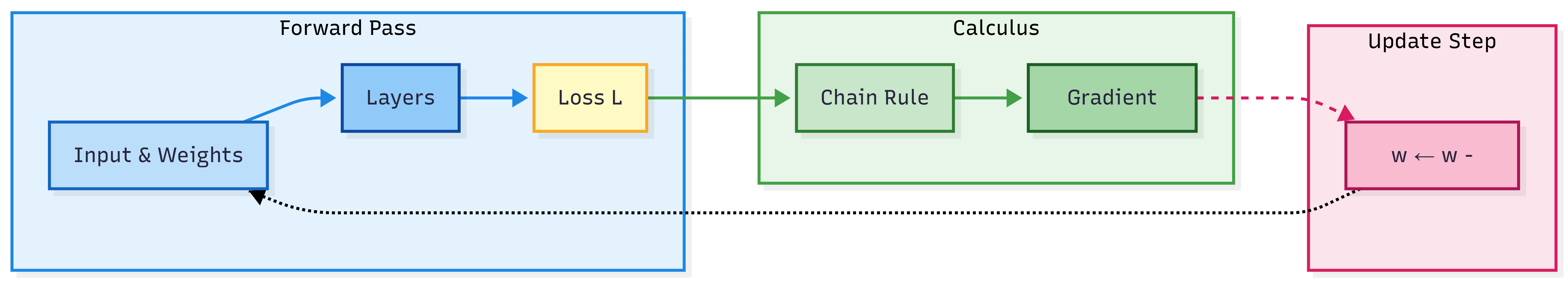
In words: Forward pass (input + weights → layers → loss). Backprop applies the chain rule to get the gradient of the loss w.r.t. all weights. Update: subtract \( \alpha \times \text{gradient} \) from weights. Repeat.

---

One-Page Cheat Sheet

Concept	Definition / formula
Derivative \( \frac{df}{dx} \)	Rate of change of \( f \) w.r.t. \( x \).
Partial derivative \( \frac{\partial f}{\partial x_i} \)	Derivative w.r.t. \( x_i \), other variables fixed.
Gradient \( \nabla f \)	Vector of partial derivatives: \( \left( \frac{\partial f}{\partial x_1}, \ldots, \frac{\partial f}{\partial x_n} \right)^T \). Points in direction of steepest ascent.
Gradient descent	\( \mathbf{w} \leftarrow \mathbf{w} - \alpha \nabla L \). Step in direction of steepest descent.
Chain rule	\( \frac{\partial L}{\partial w} = \frac{\partial L}{\partial y} \frac{\partial y}{\partial w} \) (and extend along the graph).
Backpropagation	Chain rule applied to the network; one backward pass gives gradients for all weights.
Jacobian	Matrix of partial derivatives for vector-valued \( \mathbf{f}(\mathbf{x}) \); \( J_{ij} = \frac{\partial f_i}{\partial x_j} \).
Learning rate \( \alpha \)	Step size in gradient descent; too large ⇒ unstable; too small ⇒ slow.
Stationary point	Where \( \nabla f = 0 \) (local min, local max, or saddle point).
Automatic differentiation	Compute derivatives by applying chain rule on the computational graph; exact and efficient.

---

Formula Card

Name	Formula
Derivative (limit)	\( f'(x) = \lim_{h \to 0} \frac{f(x+h) - f(x)}{h} \)
Gradient	\( \nabla f = \left( \frac{\partial f}{\partial x_1}, \ldots, \frac{\partial f}{\partial x_n} \right)^T \)
Gradient descent update	\( \mathbf{w}_{\mathrm{new}} = \mathbf{w}_{\mathrm{old}} - \alpha \nabla_{\mathbf{w}} L \)
Chain rule (two steps)	\( \frac{\partial L}{\partial w} = \frac{\partial L}{\partial y} \cdot \frac{\partial y}{\partial w} \)
Directional derivative	\( \nabla f \cdot \mathbf{v} \) (rate of change in direction \( \mathbf{v} \))
Jacobian (element)	\( J_{ij} = \frac{\partial f_i}{\partial x_j} \)

---

What’s Next

• Backpropagation — Chain rule in action: computational graphs, forward vs backward pass, and why backprop is efficient.
• Optimization Fundamentals — Convex vs non-convex, saddle points, and why gradient descent works in practice despite non-convexity.
• Optimizers — SGD, Momentum, Adam, AdamW, and learning rate schedules.
• Loss Functions — Cross-entropy, MSE, and how they connect to gradients.

You will use calculus (gradient, chain rule) in every topic that involves training: backprop, optimizers, regularization (gradient of penalty terms), and sensitivity analysis (gradient w.r.t. inputs).

---

Revision Checklist

Before an interview, ensure you can:

• Define derivative, partial derivative, and gradient. Say in which direction the gradient points (steepest ascent).
• Write the gradient descent update rule and explain why we use \( -\nabla L \).
• State the chain rule and explain how backpropagation uses it.
• Differentiate: derivative vs gradient vs Jacobian (scalar vs vector output).
• Explain why we use automatic differentiation (backprop) instead of numerical differentiation.
• Answer: “What happens when the gradient is zero?” (stationary point, not necessarily global min.)
• Avoid traps: “gradient points to minimum,” “backprop = numerical diff,” “gradient is a scalar,” “we need Hessian to train.”

---

Related Topics

• Linear Algebra for Deep Learning — Vectors, matrices; gradient is a vector, Jacobian is a matrix.
• Probability & Statistics for Deep Learning — MLE/MAP and why we minimize negative log-likelihood (loss); gradient descent as optimization.
• Backpropagation — Implementation of the chain rule for neural networks.
• Optimizers — How gradients are used by SGD, Adam, etc.