Pre-Notes: Learning Objectives & Prerequisites

Learning Objectives

By the end of this note you will be able to:

• Define an artificial neuron and the perceptron and state their mathematical formulation.
• Explain linear decision boundaries and why a single perceptron can only learn linearly separable data.
• Describe the perceptron learning rule and how it relates to optimization (gradient descent, loss minimization).
• Explain the XOR problem and why it motivated multi-layer networks and non-convex optimization.
• Give an intuition for the universal approximation theorem (what it says and why it matters).
• Connect convex vs non-convex loss, saddle points, and local vs global minima to single-neuron vs multi-layer models.
• Explain why deep learning works despite non-convexity and gradient descent as maximum likelihood in the context of neurons and loss.

Prerequisites

Before starting, you should know:

• Basic algebra: weighted sums, linear equations, inequalities.
• Idea of “learning from data”: we have inputs, outputs, and we want to find a rule that fits the data.
• Optional: Basic calculus (derivatives) and “minimizing a function” help for the optimization part.

If you don’t, review Linear Algebra for Deep Learning and Optimization Fundamentals (for the optimization sections).

Where This Fits

• Builds on: Linear Algebra (dot products, linear combinations), Optimization Fundamentals (what is optimization, gradient descent, convex vs non-convex).
• Needed for: Activation Functions, Loss Functions, Backpropagation, and all deeper architectures (MLP, CNN, RNN).

This topic is the core building block of Phase 2: Core Neural Network Internals and is the foundation of every deep learning model.

---

1. What is an Artificial Neuron & Perceptron?

An artificial neuron is the smallest computational unit in a neural network. It takes several numeric inputs, multiplies each by a weight, adds a bias, and passes the result through an activation function to produce one output.

A perceptron is a specific type of artificial neuron: a single layer of such units (or a single unit) that takes inputs, computes a weighted sum plus bias, and applies a step (threshold) activation to output a binary decision (e.g., 0 or 1). Historically, “perceptron” often refers to this binary linear classifier.

Simple Intuition

Think of a simple yes/no referee: they look at a few factors (inputs), give more importance to some (weights), have a built-in bias (bias term), and finally say “yes” or “no” (activation). The perceptron is that referee in math form: weighted votes + bias → threshold → class.

Formal Definition (Interview-Ready)

An artificial neuron computes output = activation(Σᵢ wᵢ xᵢ + b), where xᵢ are inputs, wᵢ are weights, b is the bias, and activation is a (usually non-linear) function. A perceptron is an artificial neuron (or a single layer of such neurons) that uses a step/threshold activation to produce a binary output, forming a linear binary classifier.

---

In a Nutshell

An artificial neuron = weighted sum of inputs + bias, then activation. A perceptron = same thing with a step function so the output is 0 or 1; it’s the simplest linear binary classifier.

---

2. Why Do We Need It?

We need a learnable, data-driven way to make decisions (e.g., classify into two classes) instead of hand-coding rules. The artificial neuron and perceptron give us:

• A single mathematical building block that can be repeated and stacked (layers).
• Learning by adjusting weights and bias from data (optimization).
• A bridge from linear models (perceptron) to non-linear deep networks (many neurons and layers).

Old vs New Paradigm

Paradigm	How decisions are made
Hand-crafted rules	If condition A and B then class 1
Perceptron / Neuron	Weights and bias learned from data
Deep networks	Many stacked neurons learning hierarchy

Key Reasons

• Interpretable structure: One neuron = one weighted combination + activation; easy to explain and implement.
• Foundation for depth: Stacking neurons gives multi-layer perceptrons (MLPs) and eventually CNNs, RNNs, Transformers.
• Optimization link: Training a perceptron = minimizing a loss (e.g., misclassification); this connects to gradient descent and convex optimization for the single-neuron case.

Real-World Relevance

Domain	Why neuron/perceptron matters
Classification	Perceptron is the simplest linear classifier; MLPs extend it.
Feature learning	Layers of neurons learn hierarchical features.
Theory	XOR and linear separability motivate non-linearity and depth.

---

3. Core Building Block: How It Works

Biological Inspiration

Biological neuron	Artificial neuron
Dendrites (inputs)	Input values xᵢ
Synaptic strengths	Weights wᵢ
Cell body (summation)	Weighted sum + bias
Axon (output)	Activation(output)

Mathematical Formulation

For inputs x₁, x₂, …, xₙ, weights w₁, w₂, …, wₙ, and bias b:

Pre-activation (net input):

z = w₁x₁ + w₂x₂ + … + wₙxₙ + b = w·x + b

Output:

y = activation(z)

Perceptron (step activation):

y = 1  if z ≥ 0
y = 0  if z < 0

(Some definitions use y ∈ {−1, +1}; the idea is the same: a threshold on z.)

Interview-ready: The core building block is z = w·x + b and y = activation(z). For the perceptron, activation is a step function so the decision boundary is w·x + b = 0 (a hyperplane).

---

Diagram: Artificial Neuron (Single Unit)

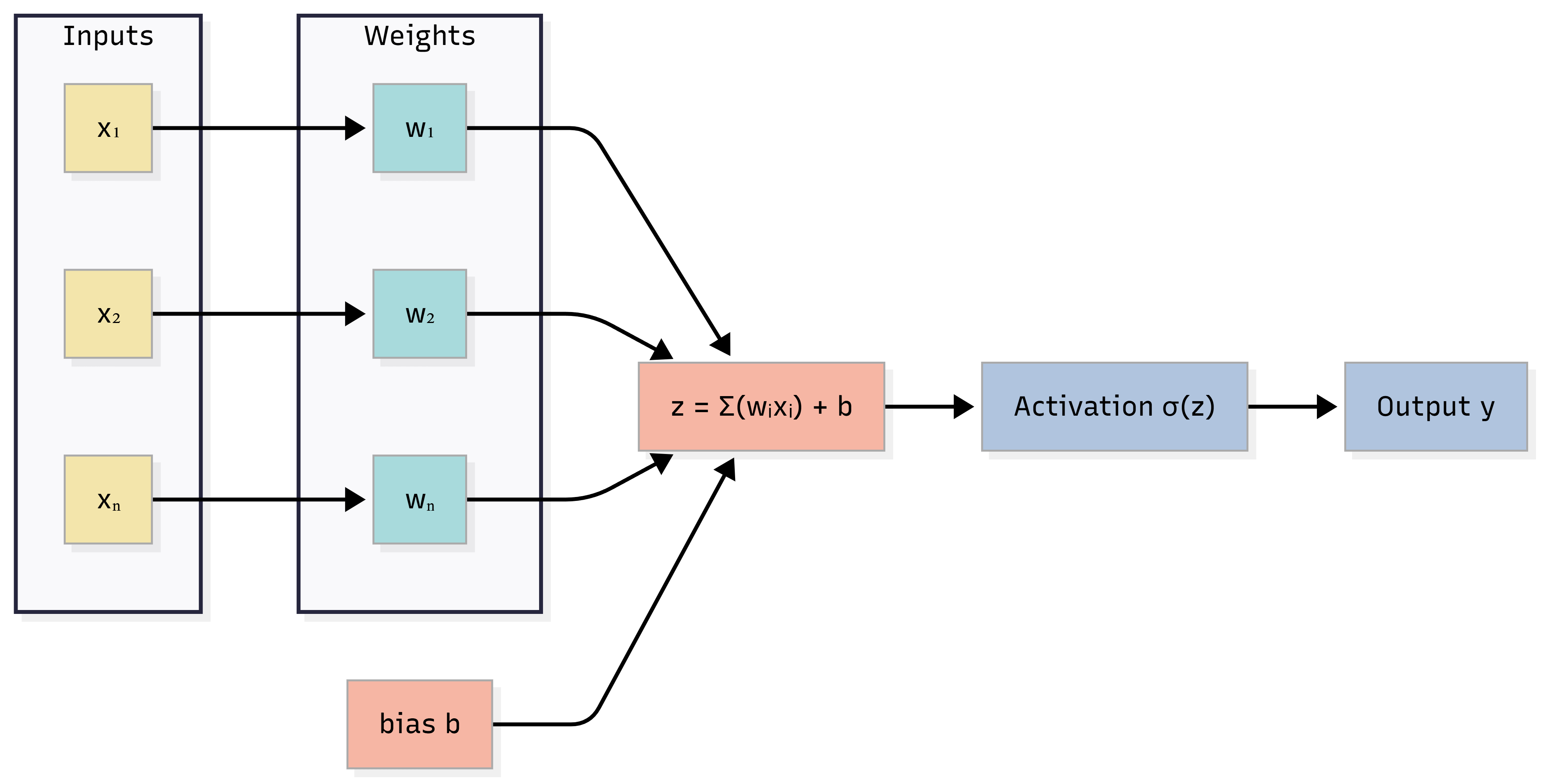
Caption: Inputs xᵢ are multiplied by weights wᵢ, summed with bias b to get z, then passed through activation to get y. For a perceptron, activation is a step function.

---

In a Nutshell

One neuron: z = w·x + b, y = activation(z). Perceptron: activation = step, so output is binary and the decision boundary is the hyperplane w·x + b = 0.

---

Think about it: If we use no activation (identity), what kind of function does a single neuron compute? What happens if we stack many such neurons in a layer?

---

4. Process: How the Perceptron Learns (Training)

Training a perceptron means finding weights and bias so that for as many training examples as possible, the predicted class matches the true class. This is an optimization process: we are effectively minimizing a loss (e.g., number of misclassifications or a surrogate loss).

Step-by-Step (Perceptron Learning Rule)

1. Initialize weights and bias (e.g., to 0 or small random values).
2. For each training example (x, target t):
   • Forward: Compute z = w·x + b, output y = step(z).
   • Compare: If y ≠ t, we have an error.
   • Update (learning rule):
     • If we predicted 0 but target was 1: w ← w + η·x, b ← b + η (push boundary so x is classified as 1).
     • If we predicted 1 but target was 0: w ← w − η·x, b ← b − η (push boundary so x is classified as 0).
3. Repeat over the dataset for multiple epochs until no errors (or convergence).

Unified form (with signed target t ∈ {−1, +1}):

• Prediction wrong ⇒ w ← w + η · t · x, b ← b + η · t.

This update is equivalent to gradient descent on a suitable loss (e.g., perceptron loss). So the perceptron learning rule is a simple form of optimization: we change parameters so that the loss decreases.

Link to Optimization

• What is optimization? Finding parameters (here w, b) that minimize a loss (e.g., misclassification error or a differentiable surrogate).
• For a single linear neuron with a suitable loss, the loss surface can be convex, so repeated updates (gradient descent / perceptron rule) can converge to a global minimum when the data is linearly separable.
• Gradient descent as maximum likelihood: When we use losses like MSE (regression) or cross-entropy (classification), minimizing that loss is equivalent to maximum likelihood estimation (MLE). The perceptron rule is a special case of such updates for a linear model with a step output.

---

In a Nutshell

Perceptron learning rule: On a misclassification, update w and b in the direction that would correct that example. This is a form of gradient-based optimization; for a single perceptron the loss can be convex when data is linearly separable.

---

5. Key Sub-Topics

5.1 Linear Decision Boundary

The equation w·x + b = 0 defines a hyperplane in the input space. Points with w·x + b ≥ 0 are classified one way (e.g., 1); points with w·x + b < 0 are classified the other (e.g., 0). So the decision boundary is linear. A single perceptron can only separate two classes if they are linearly separable.

Concept	One-line summary
Decision boundary	Set of x where w·x + b = 0 (hyperplane)
Linear separability	Two classes can be split by some hyperplane
Perceptron limit	Only works when such a hyperplane exists

5.2 Perceptron Learning Rule (Recap)

• When: Update only on misclassification.
• How: w ← w + η·t·x, b ← b + η·t (for t ∈ {−1, +1}).
• Why it works: Each update moves the hyperplane so that the misclassified point is on the “correct” side; over many passes the boundary converges (for linearly separable data).

5.3 XOR Problem

XOR (exclusive OR) is not linearly separable: you cannot draw a single straight line (in 2D) to separate the two classes. So a single perceptron cannot learn XOR.

• Implication: We need non-linearity and/or multiple layers (e.g., two layers can implement XOR). This motivated multi-layer perceptrons (MLPs) and activation functions.
• Optimization angle: A single perceptron’s loss (for linearly separable data) can be convex. Once we add hidden layers and non-linear activations, the loss becomes non-convex (many local minima, saddle points). So the XOR problem leads directly to non-convex optimization in deep learning.

5.4 Universal Approximation Theorem (Intuition)

Roughly: a feedforward network with one hidden layer and a suitable non-linear activation can approximate any continuous function on a bounded domain to arbitrary accuracy (with enough hidden units). So:

• One neuron = one hyperplane (linear).
• One hidden layer of neurons = combination of many hyperplanes + non-linearity = can approximate complex boundaries and functions.

We don’t need to prove it in an interview; knowing that “one hidden layer can approximate well” and “depth helps in practice” is enough.

5.5 Optimization in the Picture: Convex vs Non-Convex, Saddle Points, Local vs Global Minima

• What is optimization? Finding parameters that minimize a loss. For the perceptron we do this iteratively (perceptron rule / gradient descent).
• Convex vs non-convex loss: For a single linear neuron (e.g., linear regression with MSE, or perceptron with a convex surrogate loss), the loss in (w, b) can be convex: one “bowl,” and any local minimum is the global minimum. For multi-layer networks with non-linear activations, the loss is non-convex: many local minima, saddle points, and no guarantee of reaching the global minimum.
• Saddle points: A point where the gradient is zero but the loss decreases in some directions and increases in others. In high-dimensional neural networks, saddle points are common; momentum and stochasticity help escape them.
• Local vs global minima: Local = lowest in a small neighborhood; global = lowest over the whole parameter space. In non-convex settings we usually find a good local minimum, not necessarily the global one.
• Why deep learning works despite non-convexity: Many good local minima with similar loss; saddle points are escapable; overparameterization and good initialization help. We don’t need the global minimum—we need a good enough minimum that generalizes.
• Gradient descent as maximum likelihood: For common losses (MSE, cross-entropy), minimizing the loss = maximizing the likelihood of the data. So gradient descent on that loss is doing MLE for the model parameters.

---

In a Nutshell

Single perceptron → linear boundary; can only do linearly separable problems. XOR needs non-linearity / hidden layers → non-convex loss. Universal approximation says one hidden layer (with enough units) can approximate many functions. Optimization: convex for single neuron in nice cases; non-convex for MLPs; we still train well by finding good local minima and escaping saddles.

---

Self-check: Why can’t a single perceptron solve XOR? What do we need to add (conceptually) to fix that?

---

6. Comparison: Perceptron vs Related Concepts

Aspect	Perceptron	Logistic regression (single neuron, sigmoid)	Single neuron (ReLU)
Activation	Step (0/1)	Sigmoid (probability)	ReLU
Output	Binary class	Probability	Real (non-negative)
Decision boundary	Linear (hyperplane)	Linear (hyperplane)	Linear (half-space)
Training	Perceptron rule / GD	Gradient descent on cross-entropy	Gradient descent
Loss surface	Can be convex (separable)	Convex (for linear model)	Convex in (w,b) (linear)

Aspect	Artificial neuron (math)	Biological neuron
Input	Numeric vector x	Dendritic signals
Weights	w (learned)	Synaptic strengths
Summation	w·x + b	Cell body integration
Output	activation(z)	Firing rate / spike

---

7. Common Types / Variants

1. Single-layer perceptron – One output neuron with step activation; binary linear classifier. Use case: Historically the first “learning” neuron; teaching linear separability.
2. Multi-layer perceptron (MLP) – Multiple layers of neurons with non-linear activations. Use case: General function approximation; basis of modern deep nets.
3. Perceptron with sigmoid – Same z = w·x + b, but activation = sigmoid; outputs a probability. Use case: Logistic regression; binary classification with probabilities.
4. Linear neuron (no activation) – y = w·x + b. Use case: Linear regression; stacking many gives still-linear models unless we add non-linearity elsewhere.

---

8. FAQs & Common Student Struggles

Q1. What is the difference between an artificial neuron and a perceptron?

An artificial neuron is the general unit: output = activation(w·x + b) with any activation. A perceptron is typically an artificial neuron (or a layer of them) with a step (threshold) activation used for binary classification; so every perceptron is an artificial neuron, but not every artificial neuron is a “perceptron” in the classic sense.

---

Q2. Why can’t a single perceptron solve XOR?

Because XOR is not linearly separable: no single straight line (in 2D) can separate the two classes. A perceptron’s decision boundary is always a hyperplane, so it cannot represent XOR. We need multiple layers and non-linear activations.

---

Q3. Is the perceptron learning rule the same as gradient descent?

The perceptron rule (update on misclassification) is a special case of gradient descent for a particular loss (perceptron criterion). So they are related: both are optimization procedures that update w and b to reduce error.

---

Q4. What is “linear separability”?

Two classes are linearly separable if there exists a hyperplane such that all points of one class lie on one side and all points of the other on the other side. A single perceptron can only learn such a boundary.

---

Q5. What does the universal approximation theorem say?

Roughly: a feedforward network with one hidden layer and a non-linear activation can approximate continuous functions arbitrarily well (with enough hidden units). So one hidden layer is enough for “approximation power”; in practice depth helps for efficiency and generalization.

---

Q6. Why is the loss non-convex for neural networks but convex for a single linear neuron?

A single linear neuron (e.g., y = w·x + b with MSE or perceptron loss) has a loss that is convex in (w, b). Once we add hidden layers and non-linear activations, the composition of many non-linear functions makes the loss non-convex: many local minima and saddle points.

---

Q7. What is a saddle point and why does it matter for training?

A saddle point is where gradient = 0 but the loss is not a local minimum (it goes down in some directions, up in others). In high dimensions they are common. Optimizers with momentum or stochasticity can escape saddle points; pure gradient descent might get stuck briefly.

---

Q8. How is gradient descent related to maximum likelihood?

For MSE (Gaussian noise) or cross-entropy (classification), minimizing the loss is equivalent to maximizing the likelihood of the data. So gradient descent on that loss = iterative MLE for the parameters.

Interview tip: When asked “how do we train a neuron?” you can say: we define a loss, compute gradients (e.g., by backprop later), and update weights by gradient descent—and for standard losses, that’s MLE.

---

9. Applications (With How They Are Achieved)

1. Binary linear classification

Applications: Spam vs not spam, simple medical triage (e.g., one linear score).

How neuron/perceptron achieves this: One neuron with step or sigmoid activation learns w and b so that w·x + b separates the two classes. Training uses the perceptron rule or gradient descent on cross-entropy.

Example: A single perceptron (or logistic regression) classifying emails by a few hand-crafted features.

---

2. Building block for deep networks

Applications: All of deep learning (vision, NLP, etc.).

How: Every layer in an MLP/CNN/RNN is made of artificial neurons. The perceptron/neuron is the core building block; stacking and training many gives deep learning.

Example: An MLP for tabular data: input layer → hidden layers (many neurons) → output layer.

---

3. Teaching and theory

Applications: Explaining linear separability, XOR, and why we need depth and non-linearity.

How: The perceptron is the simplest model to show linear boundary, convex optimization for the single-neuron case, and limitations (XOR) that motivate non-convex multi-layer optimization.

Example: A course module “From perceptron to MLP” using XOR as the motivating example.

---

10. Advantages and Limitations (With Examples)

Advantages

1. Simple and interpretable
We can write the decision rule explicitly: w·x + b ≥ 0 ⇒ class 1. We can inspect w to see which inputs matter.

Example: A medical triage score that is a weighted sum of a few vital signs; doctors can check the weights.

2. Fast and cheap to train
For a single neuron, the loss can be convex (under standard assumptions), so optimization is well-behaved and fast.

Example: Training logistic regression (one neuron with sigmoid) on millions of samples in seconds.

3. Foundation for deep learning
The same unit—weighted sum + activation—is repeated in every layer of every modern architecture.

Example: Every layer of a Transformer or CNN is built from such units (with different connectivity and activations).

Limitations

1. Only linear decision boundaries
A single perceptron cannot learn XOR or any non-linearly separable problem.

Example: Classifying points inside a circle vs outside requires at least one hidden layer with non-linearity.

2. No feature learning
A single neuron only combines the given inputs; it does not learn new representations. Deep networks learn features in hidden layers.

Example: For images, we need convolutional layers (many neurons) to learn edges and shapes; one neuron cannot.

3. Non-convexity when we go deep
As soon as we use multiple layers and non-linear activations, the loss becomes non-convex (local minima, saddle points). Training is harder than for a single neuron.

Example: Training a 10-layer MLP: we may get stuck in saddle points or suboptimal local minima without good initialization and optimizers.

---

11. Interview-Oriented Key Takeaways

• Artificial neuron = z = w·x + b, y = activation(z). Perceptron = same with step activation → binary linear classifier.
• Decision boundary = hyperplane w·x + b = 0; single perceptron only handles linearly separable data.
• Perceptron learning rule = update w, b on misclassification; equivalent to gradient descent on a suitable loss; for single neuron, loss can be convex.
• XOR is not linearly separable → need hidden layers + non-linearity → non-convex optimization in deep learning.
• Universal approximation: One hidden layer (with enough units and non-linearity) can approximate many functions; depth helps in practice.
• Optimization: Convex for single linear neuron in standard cases; non-convex for MLPs; saddle points and local minima matter; gradient descent on MSE/cross-entropy = MLE.

---

12. Common Interview Traps

Trap 1: “Can a single perceptron learn any binary function?”

Wrong: Yes, it’s a universal classifier.

Correct: No. A single perceptron can only learn linearly separable functions. It cannot learn XOR or any non-linearly separable mapping.

---

Trap 2: “Is the perceptron learning rule the same as backpropagation?”

Wrong: Yes, they are the same.

Correct: No. The perceptron rule is an update rule for a single layer (and a specific loss). Backpropagation is a method to compute gradients in multi-layer networks. Both are used in training but do different jobs.

---

Trap 3: “If the gradient is zero, we have found the global minimum.”

Wrong: Zero gradient means we’re at the best solution.

Correct: Zero gradient means a critical point. It could be a local minimum, global minimum, local maximum, or saddle point. In non-convex optimization we don’t know which without more analysis.

---

Trap 4: “Neural network loss is convex because we use gradient descent.”

Wrong: We use gradient descent, so the loss must be convex.

Correct: Neural network loss is non-convex. We use gradient descent to find a good local minimum (or low-loss region). Convexity is not required; in practice we still get good solutions.

---

Trap 5: “More layers always mean we need non-convex optimization.”

Wrong: Only deep networks have non-convex loss.

Correct: Even one hidden layer with non-linear activation makes the loss non-convex. Depth increases complexity, but non-convexity appears as soon as we have non-linear layers.

---

Trap 6: “The goal of training is always to find the global minimum.”

Wrong: We must find the global minimum for the model to work.

Correct: In deep learning we usually cannot find or verify the global minimum. The goal is to find a good local minimum that generalizes well. Many such minima exist in overparameterized networks.

---

13. Simple Real-Life Analogy

An artificial neuron is like a committee member who takes several inputs (reports), gives each a weight (importance), adds a personal bias, and then gives a single verdict (activation). A perceptron is the strict version: the verdict is only “yes” or “no” based on whether the weighted sum crosses a threshold. The committee (one layer) can only draw a single straight line to separate two opinions; for trickier cases you need more layers (more committees) and non-linear rules.

---

14. System Design – Interview Traps (If Applicable)

Trap 1: Using a single neuron in production for a complex task

Wrong thinking: A perceptron is simple and fast, so we should use it for all binary classification.

Correct thinking: A single neuron is only appropriate when the problem is linearly separable (or approximately so). For complex boundaries, multi-layer models (and proper evaluation) are needed. In production, we also care about calibration, latency, and maintainability.

Example: Using one linear score for loan approval when risk depends on non-linear interactions (e.g., age × income) can lead to poor decisions; an MLP or tree model may be more appropriate.

---

Trap 2: Ignoring optimization behavior when scaling to MLPs

Wrong thinking: Training is “just gradient descent” whether we have one neuron or 100 layers.

Correct thinking: Single-neuron (linear) training often has convex loss; MLPs have non-convex loss (saddle points, local minima). Design choices (initialization, optimizer, learning rate, batch size) matter much more for deep networks.

Example: Default learning rate that works for logistic regression may diverge or get stuck for a 5-layer MLP without proper initialization and schedule.

---

15. Interview Gold Line

The artificial neuron is the atom of deep learning: one weighted sum plus activation. The perceptron is its simplest form—a linear binary classifier—and its failure on XOR is why we need depth and non-linearity, and thus non-convex optimization.

---

16. Self-Check and “Think About It” Prompts

Self-check 1: Write the equation of the decision boundary for a perceptron with weights w = (1, −2) and b = 3. What does “linear separability” mean in 2D?

Self-check 2: Why is the loss for a single linear neuron (e.g., MSE) convex in (w, b), but the loss for a 2-layer MLP non-convex?

Think about it: If you have 100 features and one binary label, when would you try a single perceptron first, and when would you go directly to an MLP?

Answers (concise):
- 1: Boundary: x₁ − 2x₂ + 3 = 0 (a line in 2D). Linear separability: the two classes can be separated by some straight line.
- 2: Single neuron: loss is a composition of linear map + (often convex) loss → convex in (w,b). MLP: composition of non-linear activations → non-convex.
- 3: Try perceptron when you expect a roughly linear boundary (e.g., after feature engineering); use MLP when you expect complex interactions or don’t know the structure.

---

17. Likely Interview Questions

• What is an artificial neuron? What is a perceptron?
• Write the mathematical formulation of a perceptron.
• What is a linear decision boundary? Why can’t a perceptron solve XOR?
• Explain the perceptron learning rule. How does it relate to gradient descent?
• What is the universal approximation theorem (intuition)?
• Why is the loss convex for a single linear neuron but non-convex for an MLP?
• What is a saddle point? Why does deep learning still work with non-convex loss?
• How is gradient descent related to maximum likelihood estimation?

---

18. Elevator Pitch

30 seconds:
An artificial neuron computes a weighted sum of inputs plus a bias, then applies an activation function. A perceptron uses a step function so the output is 0 or 1—it’s a linear binary classifier. It can only learn linearly separable data; XOR needs hidden layers and non-linearity, which leads to non-convex optimization. Training is done by a perceptron rule or gradient descent, which for standard losses is like maximum likelihood estimation.

2 minutes:
The artificial neuron is the building block of neural networks: z = w·x + b, y = activation(z). The perceptron is the simplest case—step activation—so the decision boundary is the hyperplane w·x + b = 0. It can only classify linearly separable data. The perceptron learning rule updates weights on misclassification and is a form of gradient descent. The XOR problem shows that one neuron is not enough; we need multiple layers and non-linear activations. That makes the loss non-convex (local minima, saddle points), but deep learning still works because there are many good minima and we can escape saddles. The universal approximation theorem says one hidden layer can approximate many functions. For common losses, gradient descent = MLE.

---

19. One-Page Cheat Sheet (Quick Revision)

Concept	Definition / formula
Artificial neuron	z = w·x + b, y = activation(z).
Perceptron	Neuron with step activation → binary output; linear classifier.
Decision boundary	w·x + b = 0 (hyperplane).
Linear separability	Two classes separable by some hyperplane.
Perceptron rule	On error: w ← w + η·t·x, b ← b + η·t (t ∈ {−1,+1}).
XOR	Not linearly separable → need hidden layers + non-linearity.
Universal approximation	One hidden layer + non-linearity can approximate many functions.
Optimization	Find (w, b) that minimize loss; e.g. gradient descent.
Convex (single neuron)	One global min; local = global.
Non-convex (MLP)	Many local minima, saddle points; no global guarantee.
GD as MLE	Minimizing MSE/cross-entropy = MLE; GD implements it.

---

20. Formula Card

Name	Formula / statement
Pre-activation	z = w·x + b
Neuron output	y = activation(z)
Perceptron (step)	y = 1 if z ≥ 0, else y = 0
Decision boundary	w·x + b = 0
Perceptron update	w ← w + η·t·x, b ← b + η·t (on misclassification, t = true label ±1)
Gradient descent	θ ← θ − η ∇L(θ)
Critical point	∇L(θ) = 0 (min, max, or saddle)

---

21. What’s Next and Revision Checklist

What’s Next

• Activation Functions: Sigmoid, Tanh, ReLU, etc.—you’ll see why we need non-linear activations (XOR, universal approximation) and how they affect gradient flow.
• Loss Functions: MSE, cross-entropy—formalize “what we minimize” and the MLE link.
• Backpropagation: How gradients ∇L(θ) are computed in multi-layer networks; the perceptron is the unit that gets repeated in every layer.
• Optimizers: SGD, Adam, learning rate schedules—same optimization ideas (convex vs non-convex, saddle points) applied to full networks.

Revision Checklist

Before an interview, ensure you can:

1. Define artificial neuron and perceptron (formula + step activation).
2. Draw the decision boundary (hyperplane) and explain linear separability.
3. State the perceptron learning rule and its link to optimization (gradient descent).
4. Explain why a single perceptron cannot learn XOR.
5. Give intuition for the universal approximation theorem.
6. Compare convex vs non-convex loss (single neuron vs MLP).
7. Explain saddle point, local vs global minimum, and why DL works despite non-convexity.
8. State that gradient descent on MSE/cross-entropy = MLE.
9. Avoid traps: “perceptron can learn any function,” “gradient zero = global min,” “NN loss is convex.”

Related Topics

• Linear Algebra for Deep Learning (dot product, hyperplanes)
• Optimization Fundamentals (convex vs non-convex, saddle points, GD, MLE)
• Activation Functions (why non-linearity)
• Loss Functions (MSE, cross-entropy)
• Backpropagation (gradients in multi-layer nets)

---

End of Artificial Neuron & Perceptron study notes.