
Linear Algebra For Deep Learning Notes
Interview-Ready Notes
Organization: DataLogos
Date: 04 Mar, 2026
Linear Algebra for Deep Learning – Study Notes
Target audience: Beginners | Goal:
End-to-end learning and interview-ready
Difficulty: Beginner-friendly (assumes basic
high-school algebra)
Estimated time: ~45 min read / ~1.5 hours with
exercises
Learning Objectives
By the end of this note you will be able to:
- Define scalars, vectors, matrices, and tensors and explain how they appear in deep learning.
- Explain matrix multiplication and dot product with geometric intuition and why they are the core of neural network computation.
- Describe rank, linear independence, and their role in understanding model capacity and singular matrices.
- Give intuition for eigenvalues/eigenvectors and their link to PCA and dimensionality reduction.
- Summarize SVD (Singular Value Decomposition) at a high level and where it appears in DL.
- Explain why tensors power DL frameworks (e.g., batch, channels, spatial dimensions).
Prerequisites
- Before starting, you should know: basic algebra (variables, equations), familiarity with coordinates and graphs.
- Helpful but not required: basic Python (for code snippets).
- Where this fits: This topic is Phase 1: Mathematical Foundations in the DL roadmap. It builds on high-school math and is needed for Calculus for Deep Learning, Backpropagation, and every architecture (ANN, CNN, RNN, Transformers).
1. What is Linear Algebra (in the Context of Deep Learning)?
Linear algebra is the branch of mathematics that studies vectors, matrices, and linear transformations. In deep learning, it is the language in which we express data, weights, and computations: every forward pass is essentially a sequence of matrix multiplications and additions.
In simple terms: linear algebra gives us the tools to handle many numbers at once—which is exactly what we do when we process batches of images, sequences of tokens, or layers of neurons.
Simple Intuition
Think of a spreadsheet where each row is a sample and each column is a feature. Linear algebra gives you rules to combine whole rows or columns at once (e.g., “multiply this block of numbers by that block”) instead of cell by cell. Neural networks do this at scale: one matrix multiply can represent millions of operations.
Formal Definition (Interview-Ready)
Linear algebra is the study of vector spaces and linear maps between them. In deep learning, we use it to represent data as vectors and matrices (or tensors), and to describe linear transformations (matrix multiplication, projections) that form the backbone of neural network layers.
2. Why Do We Need Linear Algebra for Deep Learning?
Without linear algebra we could not:
- Store and manipulate batches of data efficiently.
- Express weight matrices and biases in a compact way.
- Run parallel computation (GPUs are built to do matrix operations fast).
- Analyze rank, eigenvalues, and SVD for understanding models and reducing dimensions.
Key Reasons
| Reason | Role in DL |
|---|---|
| Efficiency | One matrix multiply does many scalar ops in one shot; GPUs optimize for this. |
| Notation | Layers are written as y = activation(Wx + b); W is a matrix, x and b are vectors. |
| Batch processing | We stack samples into a matrix (batch × features) and process the whole batch at once. |
| Dimensionality | Concepts like rank and SVD help with redundancy, compression, and PCA. |
Where Linear Algebra Shows Up in DL
| DL concept | Linear algebra used |
|---|---|
| Fully connected layer | Matrix multiplication Wx + b |
| Convolution | Strided dot products (filters as small matrices/tensors) |
| Attention scores | Dot products and softmax over vectors |
| PCA / dimensionality reduction | Eigenvectors / SVD |
| Batch normalization | Mean, variance, scaling (vectors/matrices) |
3. Core Building Block: Scalars, Vectors, Matrices, Tensors
Scalars
A scalar is a single number (e.g., a learning rate α, a loss value L). In code: a 0-dimensional tensor or a Python float.
Vectors
A vector is an ordered list of numbers, e.g. x = [x₁, x₂, …, xₙ].
- Geometric view: an arrow from the origin to the point (x₁, x₂, …).
- In DL: one sample’s features, one row/column of a batch, or a bias term.
Notation: lowercase bold x; shape (n,) or (n, 1) depending on convention.
Matrices
A matrix is a 2D grid of numbers: rows and columns.
- In DL: a weight matrix W (e.g., input_dim × output_dim), or a batch of samples (batch_size × features).
- Notation: uppercase bold A, W; shape (m, n) = m rows, n columns.
Tensors
A tensor is a generalization of scalars (0D), vectors (1D), and matrices (2D) to any number of dimensions.
- In DL: images are often (batch, height, width, channels); sequences (batch, time_steps, features). We use “tensor” and “array” loosely for multi-dimensional data.
- Why “tensor” in frameworks: PyTorch/TensorFlow use the word for any multi-dimensional array; mathematically, tensors have stricter transformation rules, but in practice we mean “n-dimensional array.”
Interview-ready: In deep learning, a tensor is a multi-dimensional array that can represent a batch of data, a single image, or the weights of a layer. The number of axes (dimensions) is often called the rank of the tensor (in the programming sense: e.g., a matrix has rank 2).
Matrix Multiplication Intuition
For a product C = AB:
- A is (m × k), B is (k × n) → C is (m × n).
- Element C[i,j] = dot product of row i of A and column j of B.
Why it matters in DL: A layer’s output is Y = XW + b: each row of X (one sample) is multiplied by W to get one row of Y. So one matrix multiply computes outputs for the entire batch.
Dot Product and Geometric Meaning
The dot product of two vectors u and v of the same length:
u · v = u₁v₁ + u₂v₂ + … + uₙvₙ
Geometric meaning:
- u · v = ‖u‖ ‖v‖ cos(θ) (θ = angle between vectors).
- If u and v are unit length,
u · v = cos(θ):
- 1 = same direction
- 0 = perpendicular
- −1 = opposite direction
In DL: Attention scores are often dot products (or scaled dot products) between query and key vectors; similarity between embeddings is frequently measured via dot product or cosine similarity.
In a nutshell: Scalars, vectors, matrices, and tensors are the “data types” of linear algebra. In DL, layers are linear maps (matrix multiply + bias) plus nonlinearity; matrix multiplication and dot products are the core operations.
4. Key Sub-Topics: Rank, Linear Independence, Eigenvalues, SVD
Rank and Linear Independence
- Linear independence: A set of vectors is linearly independent if no vector in the set can be written as a linear combination of the others.
- Rank of a matrix: The maximum number of linearly independent rows (or columns). Equals the dimension of the column space (and row space).
- Full rank: For an (m × n) matrix, rank = min(m, n). Singular (non-invertible) square matrices have rank < n.
Why it matters in DL: Low rank can mean redundant features or collinearity; singular weight matrices cause numerical issues. Rank also relates to the “effective” dimensionality of representations.
Eigenvalues and Eigenvectors (Intuition + PCA Link)
For a square matrix A, a non-zero vector v is an eigenvector if:
Av = λv
for some scalar λ (the eigenvalue). So A only stretches or flips v, it doesn’t rotate it.
PCA link: Principal Component Analysis finds directions of maximum variance in data. These directions are eigenvectors of the covariance matrix; eigenvalues indicate how much variance each direction captures. So eigenvalues/eigenvectors are the math behind PCA and many dimensionality-reduction ideas.
SVD Intuition
Singular Value Decomposition factorizes any matrix A (not necessarily square) as:
A = U Σ Vᵀ
- U and V are orthogonal matrices (rotation/reflection).
- Σ is diagonal with singular values (non-negative, often sorted decreasing).
Intuition: Any matrix can be seen as: rotate (Vᵀ) → scale along axes (Σ) → rotate again (U). The singular values tell you how much each “direction” is stretched.
In DL: SVD appears in low-rank approximation, some initialization schemes, and analyzing weight matrices; it’s also behind the math of PCA (for centered data).
In a nutshell: Rank and linear independence tell us about redundancy and invertibility; eigenvalues/eigenvectors describe stretching directions and underpin PCA; SVD generalizes this to non-square matrices and is used for compression and analysis.
5. Process / How Linear Algebra Fits the Forward Pass
A typical fully connected forward pass for one layer:
- Input: vector x (or batch matrix X).
- Linear: z = Wx + b (matrix-vector or matrix-matrix multiply + bias).
- Activation: a = activation(z) (element-wise nonlinearity).
So the “process” where linear algebra appears is: repeated linear map (matrix multiply + bias) + nonlinearity across layers. Backpropagation then uses the same objects (matrices, vectors) to compute gradients.
6. Comparison and Types
Scalars vs Vectors vs Matrices vs Tensors
| Object | Dimensions | Example in DL |
|---|---|---|
| Scalar | 0 | Learning rate, loss value |
| Vector | 1 | One sample’s features, bias |
| Matrix | 2 | Weight matrix, batch of samples |
| Tensor | 3+ | Batch of images, sequences, conv filters |
Matrix Multiplication vs Element-Wise Multiply
| Operation | Symbol / name | Use in DL |
|---|---|---|
| Matrix multiplication | AB or **@** | Layer weights × input |
| Element-wise (Hadamard) | A ⊙ B | Gates in LSTM, masking, activations |
7. FAQs & Common Student Struggles
Q1. What is the difference between a matrix and a tensor?
In programming (PyTorch, TensorFlow), “tensor” usually means any multi-dimensional array (so a matrix is a 2D tensor). In math, “tensor” has a more precise meaning (multilinear maps that transform in specific ways under coordinate changes). For DL interviews, saying “a tensor is a multi-dimensional array; matrices are 2D tensors” is fine.
Q2. Why is matrix multiplication defined the way it is (row × column)?
Because it corresponds to composing linear maps: applying A then B to a vector x gives B(Ax) = (BA)x, so the matrix of the composition is BA. The row-by-column rule is what makes this composition work.
Q3. What does the dot product tell us in deep learning?
It measures similarity (when vectors are normalized, it’s cosine similarity). In attention, high dot product between query and key means “attend more to that key.” In embeddings, similar items often have high dot product.
Q4. What is “rank” in the context of matrices?
The rank of a matrix is the maximum number of linearly independent rows (or columns). It equals the dimension of the image (column space) of the linear map. Full rank for (m×n) means rank = min(m,n). Low rank means the matrix compresses information.
Q5. How do eigenvalues relate to PCA?
PCA finds directions of maximum variance. These directions are eigenvectors of the covariance matrix; the eigenvalues are the variances along those directions. So we keep the top eigenvectors (largest eigenvalues) to reduce dimensions.
Q6. Why do we need tensors and not just matrices?
Because data in DL has more than two axes: e.g., batch × time × features for sequences, batch × height × width × channels for images. Tensors let us batch operations and keep all dimensions explicit.
Q7. What does “linear” in linear algebra mean?
A map f is linear if f(ax + by) = a f(x) + b f(y). Matrix multiplication is linear; adding a bias is an affine map (linear + translation). Neural networks are built from affine maps plus nonlinear activations.
Q8. Why are GPUs good at linear algebra?
GPUs have many cores that can do parallel arithmetic. Matrix multiplication is highly parallel: many inner products can be computed at once. So GPUs are optimized for the same operations that define neural network forward and backward passes.
Interview tip: If asked “Why linear algebra for DL?”, say: Data and weights are vectors and matrices; the forward pass is matrix multiplies and additions; GPUs are built to accelerate these operations.
8. Applications (With How They Are Achieved)
1. Fully Connected (Dense) Layers
Applications: Any ANN: classification, regression, embeddings.
How linear algebra achieves this: Each layer is y = activation(Wx + b). W and b are learned; matrix multiply Wx is the core computation.
Example: A softmax classifier: last layer matrix W maps hidden size to number of classes; one matrix multiply gives logits.
2. Convolutional Layers
Applications: Image recognition, object detection, medical imaging.
How linear algebra achieves this: Convolution is a strided dot product of a small filter (matrix/tensor) with patches of the input. The whole operation is linear (before activation); implemented as matrix multiply or direct convolution.
Example: A 3×3 conv filter is a small matrix; sliding it over the image and computing dot products at each position produces the feature map.
3. Attention Mechanism
Applications: Transformers, BERT, GPT, machine translation.
How linear algebra achieves this: Attention scores are (scaled) dot products between query and key vectors. Weighted sum of values is a linear combination. So attention is built from dot products and linear combinations.
Example: In self-attention, each token has Q, K, V; scores = QKᵀ (matrix of dot products); output = softmax(scores) V.
4. Dimensionality Reduction (PCA)
Applications: Visualization, denoising, reducing input dimension before a model.
How linear algebra achieves this: PCA uses eigenvectors of the covariance matrix (or SVD of the centered data matrix) to find directions of maximum variance. Projection onto the top eigenvectors is a matrix multiply.
Example: Reducing 1000 features to 50 by projecting onto the top 50 eigenvectors of the covariance matrix.
5. Batch Processing
Applications: Training and inference on many samples at once.
How linear algebra achieves this: Stack samples into a matrix X (batch × features). One matrix multiply XW gives outputs for the whole batch. Same formula Y = XW + b; linear algebra makes batching trivial.
Example: Forward pass for 32 samples at once: X shape (32, 784), W (784, 256) → output (32, 256).
9. Advantages and Limitations (With Examples)
Advantages
1. Compact Notation and Efficient Computation
- One equation y = Wx + b describes the whole layer; GPUs execute it in parallel.
Example: A layer with 1024×1024 weights: one matrix multiply instead of a million separate formulas.
2. Batch Processing
- Same operation for one sample or many; no loop over samples in the math.
Example: Processing a batch of 64 images through the same conv layers in one tensor operation.
3. Theory and Analysis
- Rank, eigenvalues, SVD help analyze capacity, redundancy, and stability.
Example: Using SVD to approximate a weight matrix with a low-rank version for compression.
Limitations
1. Assumes Linearity in the “Linear Part”
- Matrix multiply is linear; real-world relationships are often nonlinear. We add activations to break linearity.
Example: Without activations, a 10-layer network would still be one big linear map.
2. Scale and Numerical Issues
- Large matrices can be ill-conditioned; inverses and eigenvalues may be numerically unstable.
Example: Inverting a near-singular covariance matrix in LDA or old-style PCA can be unstable.
3. Interpretability
- High-dimensional vectors and matrices are hard to visualize; we rely on dimensionality reduction (e.g., PCA, t-SNE) to interpret.
Example: A 256-dimensional embedding is meaningful mathematically but not directly interpretable without projection.
10. Interview-Oriented Key Takeaways
- Scalars (0D), vectors (1D), matrices (2D), tensors (3D+) are the building blocks; in DL we use tensors for batches and multi-axis data.
- Matrix multiplication is the core of the linear part of a layer: y = Wx + b (or Y = XW + b for batches).
- Dot product measures similarity; in attention, scores are (scaled) dot products between queries and keys.
- Rank = number of linearly independent rows/columns; low rank ⇒ redundancy; singular matrices are non-invertible.
- Eigenvalues/eigenvectors describe stretching directions; PCA uses them for dimensionality reduction.
- SVD generalizes to any matrix (A = U Σ Vᵀ); used for low-rank approximation and analysis.
11. Common Interview Traps (Wrong vs Correct)
Trap 1: “Is a tensor the same as a matrix?”
Wrong: Yes, they’re the same.
Correct: A matrix is a 2D tensor. A tensor is a multi-dimensional array (0D = scalar, 1D = vector, 2D = matrix, 3D+ = higher-order tensor). In DL we use “tensor” for any such array.
Trap 2: “Why not just use loops instead of matrix multiplication?”
Wrong: It doesn’t matter; the math is the same.
Correct: Matrix multiplication can be executed in parallel on GPUs; loops are sequential and much slower. The same operation written as one matrix multiply is both cleaner and faster.
Trap 3: “Eigenvalues are only for square matrices, so they’re not useful for deep learning.”
Wrong: We don’t use eigenvalues in DL.
Correct: Eigenvalues are for square matrices (e.g., covariance); we use them in PCA and analysis. For non-square matrices we use SVD (singular values), which generalizes the idea and is widely used.
Trap 4: “Dot product and matrix multiplication are the same.”
Wrong: They’re the same thing.
Correct: Dot product is for two vectors of the same length (result: scalar). Matrix multiplication involves rows of the first matrix and columns of the second; one row–column dot product gives one entry of the result. So matrix multiply uses many dot products.
Trap 5: “If the weight matrix has full rank, the layer is always good.”
Wrong: Full rank means the layer is optimal.
Correct: Full rank means the linear map is invertible (for square W), but it says nothing about generalization or learning. We care about rank for numerical stability and redundancy, not as a direct quality metric.
Trap 6: “Linear algebra is only for the forward pass.”
Wrong: Backprop doesn’t use linear algebra.
Correct: Backpropagation uses the same tensors and matrices; gradients are computed with matrix calculus (Jacobians, chain rule). The backward pass is also linear algebra, just with different matrices (transposes, gradient tensors).
12. Simple Real-Life Analogy
Vectors are like addresses (list of coordinates). Matrices are like blueprints that transform one address into another. Matrix multiplication is applying one blueprint and then another. Tensors are like stacks of blueprints for different dimensions (batch, time, channels)—everything the GPU needs to do one big, parallel update.
13. Interview Gold Line
“Linear algebra is the language of deep learning: data and weights are vectors and matrices, and every layer is a linear map (matrix multiply + bias) plus nonlinearity. If you can read y = Wx + b and know why GPUs love it, you speak the language.”
Visual: How Linear Algebra Fits in One Layer
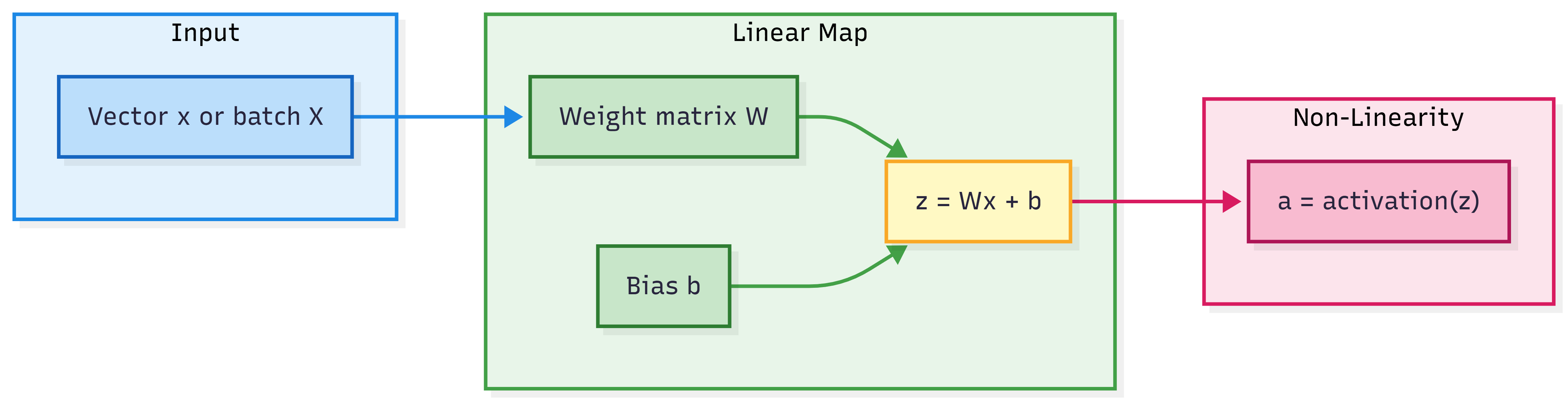
In a nutshell: One layer = linear (matrix multiply + bias) then nonlinear (activation). Linear algebra describes the linear part.
Think About It / Self-Check
Self-check: For a batch of 8 samples, each with 64 features, and a layer with 32 neurons, what are the shapes of X, W, and b? What is the shape of Y = XW + b?
Answer: X: (8, 64), W: (64, 32), b: (32,) or (1, 32); Y: (8, 32).Think about it: Why can’t a neural network with only linear layers (no activation) learn a non-linear decision boundary, no matter how many layers?
Answer: Composing linear maps gives another linear map; so the whole network would be one linear map, which can only produce linear boundaries.Think about it: In attention, we often use scaled dot product (divide by √d). Why scale?
Answer: Dot products grow with dimension d; large values push softmax into saturation and small gradients. Scaling by √d keeps scores in a reasonable range.
One-Page Cheat Sheet
| Concept | Definition / formula |
|---|---|
| Scalar | Single number (0D). |
| Vector | Ordered list of numbers (1D); shape (n,). |
| Matrix | 2D array (m × n); rows × columns. |
| Tensor | Multi-dimensional array (0D, 1D, 2D, 3D, …). |
| Dot product | u · v = Σ uᵢvᵢ; u · v = ‖u‖‖v‖ cos θ. |
| Matrix multiply | (A B)[i,j] = row i of A · column j of B; A (m×k), B (k×n) → (m×n). |
| Layer (linear part) | z = Wx + b or Z = XW + b (batch). |
| Rank | Max number of linearly independent rows (or columns). |
| Eigenvalue / eigenvector | Av = λv; λ = eigenvalue, v = eigenvector. |
| SVD | A = U Σ Vᵀ; U, V orthogonal, Σ diagonal (singular values). |
| PCA | Project onto eigenvectors of covariance matrix (largest eigenvalues). |
Takeaways:
- Data and weights in DL are vectors, matrices, tensors.
- Forward pass = repeated (matrix multiply + bias) + activation.
- Dot product = similarity; used in attention.
- Rank, eigenvalues, SVD = analysis, PCA, compression.
Formula Card
| Name | Formula |
|---|---|
| Dot product | u · v = u₁v₁ + … + uₙvₙ = ‖u‖ ‖v‖ cos θ |
| Matrix-vector multiply | (Wx)ᵢ = Σⱼ Wᵢⱼ xⱼ |
| One layer (linear) | z = Wx + b or Z = XW + b |
| Eigenvalue equation | Av = λv |
| SVD | A = U Σ Vᵀ |
| Attention scores (scaled dot product) | scores = QKᵀ / √d |
What’s Next
- Next topic: Probability & Statistics for Deep Learning (distributions, expectation, Bayes, MLE, bias–variance). You’ll use linear algebra when we define covariance matrices and PCA.
- Then: Calculus for Deep Learning (gradients, chain rule, Jacobians)—gradients of matrix expressions build directly on linear algebra.
- Later: Backpropagation and Optimizers use the same tensors and matrices for gradient flow.
Revision Checklist (Before an Interview)
Before an interview, ensure you can: